SQL for Data Analysis and AI syllabus
Course purpose
Learn to turn a business question into a checked SQL analysis and a carefully defined AI feature table. By the end, you should be able to explain why the result is valid, not only produce SQL that runs.
Audience: beginners who are comfortable with a table's rows and columns. No prior SQL, Python, Oracle, PL/SQL, machine learning or paid AI account is required. Basic arithmetic and comfort editing a text file are enough to begin. Installation is explained separately; do not assume a lab database already exists.
Dialect: PostgreSQL. Tested practice uses PGlite 0.5.9 with a PostgreSQL 18.6 WebAssembly engine. Some examples use PostgreSQL-specific casts, date_trunc and pg_input_is_valid; the latter requires PostgreSQL 16 or later. Do not expect unchanged execution on SQLite, MySQL, Oracle or SQL Server.
Suggested pace: about 14–18 hours of reading and guided practice plus 2–3 hours for the capstone; allow additional setup and review time. Study time is a design estimate, not a measured learner completion time. Take one or two modules per session and repeat exercises that reveal a gap.
Ordered learning sequence
| Module | What you will understand and be able to do | Evidence of learning |
|---|---|---|
| 1 Start with a question and a safe lab | Define a metric, identify table grain and keys, set up the synthetic lab and inspect counts | Explain 14 orders versus 19 lines; verify setup |
| 2 Select only the evidence you need | Select columns, use aliases and DISTINCT, sort reliably and take a bounded sample | Stable top-product query and distinct channel list |
| 3 Filter rows without losing the unknowns | Combine predicates, write half-open date ranges and handle NULL correctly | Boundary-aware filters and explicit unknown-city inclusion |
| 4 Calculate amounts and time periods | Use historical prices, total line discounts, CASE, date keys and safe decimal division | Hand-check line sales and a March indicator |
| 5 Summarise at a declared grain | Use COUNT, SUM and other aggregates, GROUP BY, HAVING and completeness checks | Status counts and repeat-buyer groups |
| 6 Join relationships and preserve missing matches | Use inner and left joins, key relationships and correct zero-match counts | Line descriptions and customers with no orders |
| 7 Prevent join multiplication and reconcile money | Diagnose fan-out and pre-aggregate independent children | Demonstrate and repair a doubled payment total |
| 8 Build readable analysis with subqueries and CTEs | Use scalar subqueries, EXISTS and named intermediate results | Refund-customer selection and checked net sales by channel |
| 9 Compare rows with window functions | Use frames, LAG, ranking, deterministic ties and outer filtering | Top-two customers and cautious month-over-month comparison |
| 10 Audit quality before trusting the result | Profile duplicates, normalize labels, flag invalid references and dates, apply a stated acceptance policy | Issue report and latest-valid-record result |
| 11 Prepare AI features without future leakage | Define population, cutoff, feature and label windows and preserve missingness | Six-row feature table with a leakage-risk explanation |
| 12 Use AI as a checked SQL assistant | Specify a schema contract, verify generated SQL, inspect plans and apply layered read-only safety | Repair a flawed draft and verify the correct average denominator |
| 13 Deliver a checked analysis capstone | Produce reproducible reports and a decision-useful summary with limits | Monthly report, all-customer report, audit, summary and feature appendix |
How each module works
Read the explanation before the query. Predict one or two output values. Run the named SQL file using the setup instructions. Compare the full expected result. Explain the result in ordinary language, then attempt both independent exercises in the starter files. The separate solutions include reasoning, not just answer code.
Each module connects to the previous one. Subqueries used for the fan-out repair are introduced as derived tables in module 7 before deeper CTE work in module 8. No stored procedure, trigger, package or Oracle-specific PL/SQL knowledge is required. This course focuses on analytical SELECT queries and the evidence behind them.
Assessment and boundaries
Use the ASSESSMENT.md rubric. A pass requires correct grains, populations, date boundaries, monetary reconciliation and safe handling of SQL; these are not optional style points. The capstone uses a small synthetic retail ledger and is not a real company analysis. The AI feature exercise teaches extraction design, not model training or production ML readiness.
The scope does not include database administration, index tuning at scale, transactions that move real money, production deployments, vector databases, stored programming or automatic execution of AI-generated SQL. Those require additional prerequisites and operational controls.
Alignment with the public course page
The live page reviewed on 14 October 2026 describes a planned course for people working with structured data and lists comfort with tables, rows and columns as preparation. It does not currently publish a detailed syllabus. This 13-module sequence is a proposed complete teaching design for that stated goal. An older search-indexed catalogue mentioned 13 modules, but it is not treated as the current authoritative outline. See SOURCES.md.
Set up the SQL practice lab
Choose one route
Route A is the tested self-contained local route. It needs Node.js and npm but no database server. Route B is optional for someone who already has an isolated PostgreSQL practice database. No paid hosting, AI account or cloud database signup is required.
The course's offline HTML opens in a normal browser, but it does not execute SQL. No embedded browser SQL lab is claimed or supplied.
Route A with Node and PGlite
- Extract the entire ZIP into a folder you can write to. Keep the relative folders together. Do not run directly from an archive preview.
- Install a supported Node.js LTS version, version 22 or newer, from https://nodejs.org/en/download if Node is not already installed. npm is included with the standard Node installer. Follow your computer's installation permission requirements. The authoring validation used Node 24.19.0; Windows, macOS and other Node versions have not been independently tested here.
- Open Terminal on macOS/Linux or PowerShell on Windows. Change into the extracted sql-data-ai-course folder. Use your actual extraction location, for example cd followed by a quoted folder path.
- Check the tools:
node --version
npm --version
- Install the exact locked practice dependency from the official npm registry:
npm ci
This downloads PGlite into the course folder and does not ask for a database account. It needs internet on the first run. Do not substitute an unrelated package or a random download site. If your workplace restricts installations, ask your administrator rather than bypassing the policy.
- Run the setup smoke check:
node tools/run.mjs sql/examples/01_profile.sql
Expect customers 8, order_items 19, orders 14, payments 16 and refunds 4. Column spacing may differ from the printed guide.
- Run a lesson and then your own exercise:
node tools/run.mjs sql/examples/02_select.sql
node tools/run.mjs sql/exercises/02a.sql
The starter contains only comments until you add your SQL in a text editor. An empty result from an untouched starter is not a failure or a completed exercise. Save your changes and rerun the command. End a statement with a semicolon. The path in the command is relative to your terminal's current folder.
- Run the reference checks:
npm test
The validator executes reference queries and expected failures against a new in-memory fixture, then writes validation/latest-run.json. It does not grade your free-form exercise files or written capstone. A passing reference suite proves the supplied baseline is reproducible; compare your own outputs and explanations separately.
What the runner does
Each invocation creates a fresh in-memory PGlite database, loads sql/00_setup.sql, begins a READ ONLY transaction with a five-second statement timeout and executes the requested file. Nothing needs resetting between normal runs, and changes do not persist. The schema name is always aabha_sql. No database credentials are required.
The runner is for reviewed course SQL. It is not a secure sandbox for hostile scripts: a script can contain transaction control, functions or other operations that a simple read-only wrapper cannot make harmless. Never point this runner or an AI tool at an existing production connection. The course does not grant permission to install software or access databases on a managed device.
Route B with an existing isolated PostgreSQL installation
Prerequisites: PostgreSQL 16 or later, the psql client or a compatible query editor, and a dedicated empty practice database you own. Installation of a native server is not automated by this package and was not tested. Use official installation guidance at https://www.postgresql.org/download/ if you choose this route.
In a dedicated practice database, open and execute sql/00_setup.sql once. In psql, the command below assumes you already have a connection configured and a database named aabha_practice. Replace the database name only with your verified practice database. Let psql prompt securely if your local authentication requires it; do not paste a password into a command or chat.
psql -X -v ON_ERROR_STOP=1 -d aabha_practice -f sql/00_setup.sql
psql -X -v ON_ERROR_STOP=1 -d aabha_practice -f sql/examples/02_select.sql
The setup script creates the aabha_sql schema and tables, so it requires write privileges in that practice database. It deliberately fails if the schema already exists and does not drop existing objects. If you need a reset, use a new empty practice database or ask the owner to confirm a safe reset; do not delete an unfamiliar schema.
For analysis in a query editor, start a read-only transaction, set a timeout, paste the reviewed SELECT query, then end with ROLLBACK:
BEGIN READ ONLY;
SET LOCAL statement_timeout = '5s';
-- Paste one reviewed course SELECT query here.
ROLLBACK;
After any error inside a transaction, run ROLLBACK before beginning a new transaction. Some editors run statements in separate sessions or manage transactions themselves; check the editor's behavior. A separate least-privilege read account is an additional production control, not something this exercise configures.
Troubleshooting
| Symptom | Check and action |
|---|---|
| node or npm not found | Finish official Node installation, then reopen the terminal and recheck versions |
| Cannot find package @electric-sql/pglite | Run npm ci from the folder containing package.json |
| Cannot find the SQL file | Confirm the current folder and exact relative file path; quote paths with spaces |
| Schema aabha_sql already exists | You probably ran native setup twice; use a new isolated practice database, not a blind DROP command |
| Relation does not exist | Use the aabha_sql prefix; on native PostgreSQL confirm setup was run in this same database |
| Function pg_input_is_valid does not exist | Use the pinned PGlite route or PostgreSQL 16+; do not silently substitute an unsafe date cast |
| Permission denied | Stop and check database or installation permissions with the owner; do not broaden privileges blindly |
| Transaction is aborted | Run ROLLBACK in your native editor before retrying |
| Query hits the timeout | Inspect the joins and conditions first; these tiny examples should not need a longer timeout |
| Amounts have different trailing zeros | Compare numeric values and the query's meaning; rendering of exact numeric scale can differ |
If a query differs, compare keys and values, not just the printed alignment. Expected-output CSVs use the literal marker NULL for missing values; that marker is an output convention, not the stored text 'NULL'.
Synthetic retail data dictionary
All records are invented for this course. No actual customers, merchant, payments or private source were used. Dates span 1 January through 31 March 2025 for the analysis; signup dates include late 2024. Currency is INR. Monetary columns are exact numeric(10,2). No taxes, delivery charges, costs, exchange rates or marketing attribution are modeled.
Tables and keys
| Table | Grain and key | Important columns and meaning |
|---|---|---|
| customers | One customer; customer_id | customer_name is synthetic; city can be NULL; signup_date is the registration date |
| products | One current catalogue product; product_id | category groups products; list_price is current catalogue price, not historical sales price |
| orders | One order; order_id | customer_id references customers; order_date is a date without a time zone; status is completed, pending or cancelled; channel is web or app |
| order_items | One product line on one order; (order_id,line_no) | quantity is a positive integer; unit_price is the historical per-unit price; line_discount is the total discount for the whole line |
| payments | One payment attempt; payment_id | amount is positive; only status succeeded contributes to collection; failed attempts remain evidence but not money collected |
| refunds | One recorded refund event; refund_id | amount is positive and relates to an order; more than one refund may belong to an order |
| raw_orders | One received row; batch_row | source_order_id may repeat; order_date_text and status_text are unvalidated; amount and customer_id may be missing or invalid; loaded_at orders versions |
order_items, payments and refunds are independent child tables of orders. They must be separately reduced to compatible grain before combining monetary measures. customer_name, city, product_name and monetary amount are not unique identifiers.
Metric contract
- Quarter: order_date >= 2025-01-01 and order_date < 2025-04-01
- Included orders: completed only
- Line sales before refunds: quantity * unit_price - line_discount
- Order sales before refunds: sum line sales across the order
- Included refunds: refund_date < 2025-04-01 on included orders
- Net sales: order sales before refunds minus included order refunds
- Monthly attribution: order_date month, including the order's recorded refunds
- Net average order value: net sales / completed orders in the same population
- Buying customers: distinct customer_id among included orders in that period
- All-customer contribution report: retain every customer, including zero completed-order customers
These are course definitions rather than financial-reporting rules. Payment collection, net sales and cash-flow-by-event-date are different measures. The synthetic dataset contains no late-arriving records. For historical examples, the stored completed status is assumed known on order_date; a real as-of analysis needs status history and availability times.
Known fixture checks
| Check | Value |
|---|---|
| Curated customers | 8 |
| Products | 5 |
| Orders | 14 |
| Order lines | 19 |
| Payment attempts | 16, of which 13 succeeded and 3 failed |
| Refund events | 4 |
| Raw intake rows | 8 |
| Completed orders in quarter | 11 |
| Sales before refunds on completed orders | INR 5860.00 |
| Recorded refunds on included orders | INR 215.00 |
| Quarter net sales | INR 5645.00 |
The source CSV files are readable evidence and optional import material. The setup SQL is the canonical runnable fixture. CSV nulls are represented as empty fields; expected-result CSVs use NULL as a visible missing-value marker. Do not confuse the two conventions.
Raw intake acceptance policy
Choose the latest received row for each source_order_id by loaded_at descending and batch_row descending. Then require a non-null source identifier, known customer, non-null nonnegative amount, normalized status in the accepted domain and a date parseable by PostgreSQL. Keep invalid latest records for review instead of silently taking an older version. No raw rows are deleted by the course queries.
This policy accepts batch rows 2 and 8. It does not establish source completeness, factual accuracy, freshness or a strict date-format contract. In particular, PostgreSQL date parsing accepts more formats than ISO YYYY-MM-DD; add a separately specified format rule if required.
Module 1 of 13
01 Start with a question and a safe lab
Estimated study time: 60–90 minutes. Read, predict, run, explain, then attempt the independent work.
A store manager asks, “How did sales change this quarter?” SQL can retrieve the records needed for an answer, but the question is not yet precise enough to code. Does sales mean orders placed, money collected, or the value left after refunds? Does a cancelled order count? When did the quarter end? An analyst's first job is to turn those questions into a definition another person could repeat.
This course follows a fictional small retailer through January to March 2025. Every name and transaction is invented. We will use the same records throughout so that a new SQL idea solves a familiar problem. Our final report includes completed orders placed from 1 January up to, but not including, 1 April. It subtracts refunds recorded before 1 April and assigns them to the original order month. That is a defined course metric, not accounting advice or a universal revenue rule. The currency is INR; taxes, shipping and costs are outside the dataset.
What a database gives you
A table stores rows with named columns. A row in customers describes one customer; a row in orders describes one order. A column has a type: an integer for a count or identifier, text for a label, date for a calendar date, and numeric for an exact decimal amount. A database enforces some rules about those values and lets you ask reproducible questions across tables. A query is the instruction; its result is another table-like set of rows. Retrieving a result does not change the source table.
The most useful sentence to write about any table is “One row represents ...”. This is its grain. One order can contain several product lines, and one order can be paid in installments. Therefore orders, order_items and payments do not have the same grain. Counting lines answers a different question from counting orders. This difference will later explain why a perfectly valid join can produce a wrong sales total.
A primary key identifies a row uniquely. orders has order_id as its key. order_items uses the pair order_id and line_no because line 1 can occur on many orders. A foreign key links a child row to an existing parent, such as orders.customer_id to customers.customer_id. The key states a relationship, not a business conclusion: it does not say that every customer has ordered or that every order has been paid.
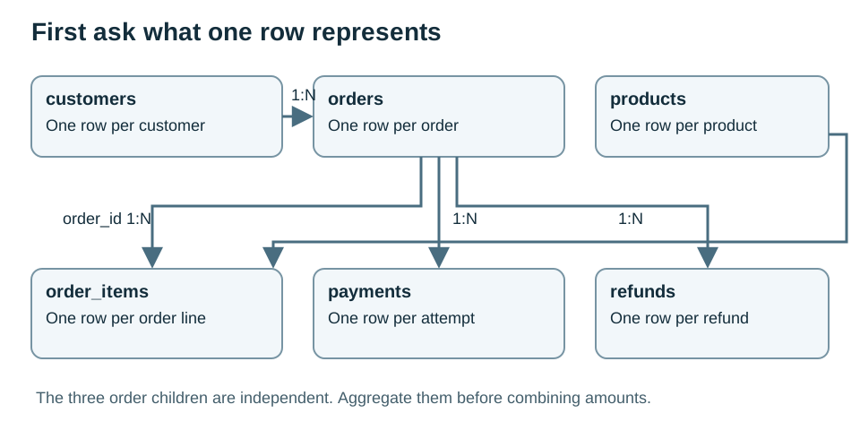
Make a safe practice space
Follow SETUP.md now. The recommended path installs one pinned package and runs a private in-memory PostgreSQL-compatible lab through Node. It does not require a PostgreSQL server, a cloud account or payment. Each run starts from the same synthetic data. The alternative instructions are for people who already have a separate PostgreSQL practice database. Do not load the setup script into a work or production database.
The setup script creates a dedicated schema named aabha_sql. The dot in aabha_sql.orders means “orders inside this schema”; it is not a file path. The lab deliberately keeps setup separate from analysis: setup creates and fills tables, while the lesson queries read them. Later we will examine read-only transactions and why they are only one safety layer.
For your first inspection, COUNT() means “count the input rows.” In a query such as SELECT COUNT() FROM aabha_sql.orders, SELECT specifies the answer and FROM names the table. COUNT(DISTINCT order_id) counts different non-null identifiers. Compare those two counts to test a proposed one-row-per-order result. Equality alone does not establish that every expected order is present, so we will also test coverage and totals.
Worked example 01 profile
Run this supplied setup check without needing to write it yet. Each SELECT counts one table; UNION ALL stacks the small answers without removing any. We revisit aggregation in module 5. Expect 8 customers, 14 orders, 19 lines, 16 payments and 4 refunds. If the counts differ, fix setup before continuing.
SELECT 'customers' AS table_name, COUNT(*) AS row_count FROM aabha_sql.customers
UNION ALL SELECT 'orders', COUNT(*) FROM aabha_sql.orders
UNION ALL SELECT 'order_items', COUNT(*) FROM aabha_sql.order_items
UNION ALL SELECT 'payments', COUNT(*) FROM aabha_sql.payments
UNION ALL SELECT 'refunds', COUNT(*) FROM aabha_sql.refunds
ORDER BY table_name;
Expected result from the bundled dataset:
| table_name | row_count |
|---|---|
| customers | 8 |
| order_items | 19 |
| orders | 14 |
| payments | 16 |
| refunds | 4 |
The runnable file is sql/examples/01_profile.sql.
Independent practice
01a
Count rows and distinct order_id values in orders. Name the outputs rows and distinct_orders. Explain what matching counts support and what they do not prove.
Hint: Use the two COUNT forms introduced above; do not join another table.
01b
Count the rows in order_items as order_lines. Use the schema diagram to explain why this number differs from the number of orders.
Hint: A basket can contain more than one product line.
Check before moving on
You can open the guide, run a supplied query, state the grain of all six curated tables, and explain why an order count is not a line count. If your setup fails, use the troubleshooting section rather than continuing with guessed results.
Module 2 of 13
02 Select only the evidence you need
Estimated study time: 45–60 minutes. Read, predict, run, explain, then attempt the independent work.
The manager first wants to see which customers exist. We do not need a total yet; we need a trustworthy sample. SQL's SELECT clause chooses columns, and FROM identifies the source. A comma separates expressions in the output. A semicolon ends the statement. SQL keywords are conventionally uppercase here to make the structure visible; unquoted PostgreSQL identifiers are folded to lowercase.
A query can rename an output with AS. In the first example, customer_name AS name makes the result heading shorter without renaming the stored column. An alias belongs to that query result. It does not add a field to the database. Similarly, selecting customer_id and city does not delete the other customer fields. Think of SELECT as choosing a view of the existing evidence.
A sample needs a stable order
Tables have no guaranteed presentation order. Even when rows appear in insertion order today, a different plan or maintenance operation can change what appears first. ORDER BY customer_id makes the result predictable. ASC is ascending and is the default; DESC puts larger values first. When two rows can tie, add a unique identifier as a final ordering key. A price ordering with product_id as a tie-breaker gives a repeatable top two even when prices match.
LIMIT takes the first specified number of rows after ordering. It helps inspect a sample; it does not prove that omitted records are clean. It also does not guarantee that the database will avoid expensive work earlier in the query. A result with LIMIT 10 can still require a large join or sort. Performance and accuracy are separate questions.
SELECT * is convenient when first inspecting a small table because the star requests all columns. For a saved analysis, list the intended columns. This documents the contract, reduces accidental exposure of unnecessary fields, and avoids a report silently changing when a new column is added. In this course the names are synthetic, but the habit matters when real data contains addresses or other private information.
Discover categories without deleting records
DISTINCT removes duplicate result rows. If you select only city, all Pune occurrences become one city label. If you select city and customer_id together, each different pair remains. DISTINCT therefore works on the full selected row, not one secretly special column. It is useful for examining categories, but it is not a general repair for duplicated business events.
NULL represents an unknown or missing value. In the city list it remains a separate result value. NULLS LAST makes its display position explicit. You have not yet decided why the city is missing or what business action is appropriate; you have only made the absence visible. Module 3 will show why filtering a missing value needs special treatment.
A good first inspection ends with a sentence: “This result contains one row per customer, sorted by customer_id, and limited to three rows.” That sentence states grain and selection. Practice writing it before running the examples. If the result's columns or number of rows cannot support the sentence, revise the query or the claim.
Worked example 02 select
Read the statement from the source table to the chosen columns, then the ordering and the limit. Predict the three identifiers before running it. The alias changes only the heading.
SELECT customer_id, customer_name AS name, city
FROM aabha_sql.customers
ORDER BY customer_id
LIMIT 3;
Expected result from the bundled dataset:
| customer_id | name | city |
|---|---|---|
| 1 | Asha | Pune |
| 2 | Ben | Bengaluru |
| 3 | Chen | Mumbai |
The runnable file is sql/examples/02_select.sql.
Worked example 02 distinct
This answers “Which city labels appear?” rather than “How many customers live in each city?” The missing city remains visible.
SELECT DISTINCT city FROM aabha_sql.customers ORDER BY city NULLS LAST;
Expected result from the bundled dataset:
| city |
|---|
| Bengaluru |
| Delhi |
| Mumbai |
| Pune |
| NULL |
The runnable file is sql/examples/02_distinct.sql.
Independent practice
02a
Return the two most expensive products with product_id, product_name and list_price. Sort descending by list_price, then ascending by product_id.
Hint: A stable tie-breaker belongs after the main ordering expression.
02b
List each distinct sales channel once in alphabetical order.
Hint: Choose only channel before applying DISTINCT.
Check before moving on
Explain why an unordered LIMIT is not a reliable top-N report, and why DISTINCT city and DISTINCT city, customer_id have different meanings.
Module 3 of 13
03 Filter rows without losing the unknowns
Estimated study time: 60–75 minutes. Read, predict, run, explain, then attempt the independent work.
The manager narrows the request to completed orders in February. A WHERE clause keeps rows that satisfy a condition. It operates on individual input rows before grouping. Equality uses =; inequality can use <>; comparisons also include <, <=, > and >=. Text values use single quotes, such as 'completed'. An unquoted word is interpreted as an identifier, not a text label.
The February condition combines three requirements with AND: the order is completed, the date is at least 1 February, and the date is before 1 March. All must be true. This half-open interval includes the start and excludes the next period's start. It is a reusable reporting pattern because adjacent periods do not overlap. With timestamps, it also avoids assuming that a day ends at 23:59:59. Our dates are plain calendar dates; a real timestamp report additionally needs an agreed time zone.
OR means either condition can be true. Mixing AND and OR without parentheses is a common way to admit unintended rows. SQL evaluates AND more tightly than OR, so make the intended groups visible. The Boolean example requires a completed order and then permits either an app order or customer 1. Without the parentheses, an OR condition at the end can bypass an earlier completion requirement.
Missing data has a third truth state
NULL is not the text 'NULL', an empty string, or zero. It means the value is missing or unknown. A comparison such as city = NULL produces unknown, not true. WHERE keeps only true rows, so that comparison will not find Farah. Use IS NULL to ask whether a value is absent and IS NOT NULL to ask whether it is present.
The same rule explains a quieter error: city <> 'Pune' does not include customers whose city is unknown. You cannot infer that a missing city is elsewhere. If the question explicitly means “not known to be Pune, including unknown cities,” write the two cases using OR city IS NULL. The words in the question decide whether that is appropriate.
COALESCE chooses the first non-null argument. In a display column, COALESCE(city,'Unknown') gives a useful label without changing the stored field. It does not establish that an unknown city is a genuine geographical category. Keep the original null semantics in mind when calculating completeness rates or joining to location data. Do not silently replace missing money with zero unless the source and metric make zero a valid interpretation.
Build a filter you can explain
Start with the smallest condition and inspect its output. Then add the date range, then any extra channel rule. Check records exactly on the boundaries. In this fixture 1005 is on 1 February, 1008 is on 28 February, and 1009 is on 1 March. A correct February filter should retain the first two and exclude the third. Checking only a middle-of-month order would miss the boundary defect.
Before using a filter in a larger report, write a plain-English inclusion rule and identify a counterexample. A cancelled app order is a useful counterexample to a misplaced OR. A missing city is a useful counterexample to an ordinary comparison. These small, deliberate tests are more informative than asking an AI tool whether the query looks correct.
Worked example 03 filter
The typed DATE literals make the intended data type explicit. The ::text cast affects the displayed date format for our runner; it does not change the filter.
SELECT order_id, customer_id, order_date::text AS order_date
FROM aabha_sql.orders
WHERE status = 'completed'
  AND order_date >= DATE '2025-02-01'
  AND order_date < DATE '2025-03-01'
ORDER BY order_date, order_id;
Expected result from the bundled dataset:
| order_id | customer_id | order_date |
|---|---|---|
| 1005 | 4 | 2025-02-01 |
| 1006 | 2 | 2025-02-14 |
| 1008 | 6 | 2025-02-28 |
The runnable file is sql/examples/03_filter.sql.
Worked example 03 nulls
The filter uses IS NULL on the source value. COALESCE is only used to label the returned result.
SELECT customer_id, customer_name, COALESCE(city,'Unknown') AS city_label
FROM aabha_sql.customers WHERE city IS NULL ORDER BY customer_id;
Expected result from the bundled dataset:
| customer_id | customer_name | city_label |
|---|---|---|
| 6 | Farah | Unknown |
The runnable file is sql/examples/03_nulls.sql.
Worked example 03 logic
Check that cancelled app order 1013 is absent. It satisfies the app condition but fails the completed condition.
SELECT order_id, status, channel FROM aabha_sql.orders
WHERE status = 'completed' AND (channel = 'app' OR customer_id = 1)
ORDER BY order_id;
Expected result from the bundled dataset:
| order_id | status | channel |
|---|---|---|
| 1001 | completed | web |
| 1002 | completed | app |
| 1005 | completed | app |
| 1009 | completed | app |
| 1010 | completed | web |
| 1012 | completed | app |
| 1014 | completed | app |
The runnable file is sql/examples/03_logic.sql.
Independent practice
03a
Return order_id and status for noncompleted orders in February 2025, ordered by order_id.
Hint: Apply the same half-open date range and change the status condition.
03b
Return customer_id and customer_name for customers in Pune or with a missing city, ordered by customer_id.
Hint: Unknown city is an explicit second case, not an inequality.
Check before moving on
You can predict whether an unknown comparison is retained by WHERE, and explain why February excludes order 1009 even though it is completed.
Module 4 of 13
04 Calculate amounts and time periods
Estimated study time: 60–75 minutes. Read, predict, run, explain, then attempt the independent work.
A stored price is not yet a sales amount. Each order line contains a quantity, a historical unit_price and a line_discount. In this dataset line_discount is one total discount for the entire line, not a per-unit discount. The agreed line calculation is quantity multiplied by unit_price, minus line_discount. Read the data dictionary before writing arithmetic; multiplying the discount by quantity would answer a different question.
The products table contains a current list price. It is useful for describing the catalogue, but past order sales must use order_items.unit_price. In a real shop, prices change. Joining today's list price into an old order can rewrite history without changing a single stored transaction. This is an example of why knowing column meaning matters more than knowing syntax.
PostgreSQL numeric stores exact decimal values at the declared precision. That is appropriate for this small financial-style fixture. Floating-point types approximate many decimal fractions and can introduce small representation differences. Integers are appropriate for whole quantities. If both sides of division are integers, PostgreSQL integer division truncates the fractional part. A decimal such as 100.0 makes the percentage calculation decimal. Round only the final displayed measure unless the business definition explicitly rounds each transaction.
Label values with CASE
CASE evaluates conditions and returns an expression. WHEN line_discount > 0 THEN 'discounted' identifies discounted lines; ELSE 'full_price' labels the remainder. END closes the expression. This adds a result column; it does not edit the source data. The order of WHEN branches matters because the first true branch wins. Choose branches that match the policy and make the fallback explicit, especially if unknown values are possible.
To select a short list of identifiers, IN (1004,1006) means that the value matches either listed identifier. It is a compact alternative to joining equality conditions with OR. The list uses numbers here; text values in a list would need single quotes.
A CASE expression is also useful for binary features: 1 for an event inside a period and 0 outside it. A binary result is just a defined indicator, not a prediction. If a future model uses it, the event must have been observable before the prediction time. We will return to that distinction in module 11.
Make time labels precise
The month key in this course is the first date of the month, created using date_trunc('month',order_date) and cast to date. Grouping by a full date key preserves the year. Grouping only by the month number would mix January 2025 with January 2026. A final ::text conversion is for stable text output in the practice runner.
Subtracting one PostgreSQL date from another returns the number of days between them. We use a fixed cutoff instead of the machine's current date, so your result will match the worked answer next year. This is a reproducibility choice. If an operational report uses today, record its run date and time zone alongside the result.
Undefined is not automatically zero
A percentage needs a numerator, denominator and population definition. NULLIF(denominator,0) returns NULL when the denominator is zero, which avoids a division-by-zero error. The resulting null percentage means the rate is undefined. Replacing it with zero would claim an observed zero rate even though there was no denominator. That may be appropriate for some displays, but it must be a separate, explicit presentation policy.
Check one calculation by hand before trusting the full output. For order 1006, the bag contributes 800 minus 80, and three pens contribute 3 times 40. The total is 840. A single hand calculation will not prove the entire report, but it catches a mistaken discount unit early.
Worked example 04 calculate
The arithmetic runs independently for each line. The CASE column explains the branch taken without altering any values.
SELECT order_id, line_no,
 quantity * unit_price - line_discount AS line_sales,
 CASE WHEN line_discount > 0 THEN 'discounted' ELSE 'full_price' END AS price_type
FROM aabha_sql.order_items WHERE order_id IN (1004,1006)
ORDER BY order_id,line_no;
Expected result from the bundled dataset:
| order_id | line_no | line_sales | price_type |
|---|---|---|---|
| 1004 | 1 | 120.00 | full_price |
| 1004 | 2 | 400.00 | discounted |
| 1006 | 1 | 720.00 | discounted |
| 1006 | 2 | 120.00 | full_price |
The runnable file is sql/examples/04_calculate.sql.
Worked example 04 dates
The January 31 order maps to January 1, and March 31 is one day before April 1. These are useful boundary checks.
SELECT order_id, date_trunc('month',order_date)::date::text AS order_month,
 DATE '2025-04-01' - order_date AS days_before_cutoff
FROM aabha_sql.orders WHERE order_id IN (1001,1004,1012)
ORDER BY order_id;
Expected result from the bundled dataset:
| order_id | order_month | days_before_cutoff |
|---|---|---|
| 1001 | 2025-01-01 | 86 |
| 1004 | 2025-01-01 | 60 |
| 1012 | 2025-03-01 | 1 |
The runnable file is sql/examples/04_dates.sql.
Worked example 04 ratio
Compare a valid denominator with zero. The null result is intentional evidence of an undefined rate.
SELECT ROUND(100.0 * 3 / NULLIF(14,0),2) AS example_percent,
 100.0 * 3 / NULLIF(0,0) AS undefined_percent;
Expected result from the bundled dataset:
| example_percent | undefined_percent |
|---|---|
| 21.43 | NULL |
The runnable file is sql/examples/04_ratio.sql.
Independent practice
04a
For order 1005 return before_discount, line_discount and line_sales. Explain in a sentence why the discount is subtracted once.
Hint: The discount belongs to the whole line.
04b
For orders 1008, 1009 and 1012 return order_id and in_march, using CASE to produce 1 for dates in March and 0 otherwise.
Hint: Use the date boundaries taught in module 3. IN (1008,1009,1012) is shorthand for matching any of those identifiers.
Check before moving on
You can distinguish a historical transaction price from a catalogue price, a line discount from a unit discount, and an undefined percentage from zero.
Module 5 of 13
05 Summarise at a declared grain
Estimated study time: 60–90 minutes. Read, predict, run, explain, then attempt the independent work.
A row-level query can show every order, but a manager often needs one row per channel or month. GROUP BY changes the output grain. It collects rows with the same grouping values so aggregate functions can reduce each collection to a measure. COUNT counts, SUM adds, AVG averages, and MIN and MAX choose the smallest or largest non-null value. An aggregate without GROUP BY summarises the whole selected input.
The first example starts with completed orders, groups them by channel, and counts the rows in each group. Because orders already has one row per order, COUNT(*) means completed orders here. The same expression over joined order lines would mean lines instead. There is no universal “count orders” function that repairs an incorrect input grain for you.
A grouped result should select its grouping keys and aggregate expressions. Asking for an unrelated detail such as order_id in a one-row-per-channel report is ambiguous: which order would represent the channel? PostgreSQL rejects many such combinations. Rather than treating the error as a nuisance, use it to reconsider what one output row is supposed to mean.
WHERE and HAVING answer different questions
WHERE filters source rows before the groups are made. HAVING filters complete groups after their aggregates exist. To ask for channels with at least five completed orders, first remove noncompleted rows with WHERE, then use HAVING COUNT(*) >= 5. Putting the status condition only in a later layer could mix cancelled or pending orders into the count.
An alias created in SELECT is not generally available to WHERE or HAVING at the same query level. Write the aggregate in HAVING or use a later query layer, introduced in module 8. The conceptual flow diagram is a reasoning aid, not a promise about the physical execution plan. A database optimizer may implement an equivalent computation in a different order.
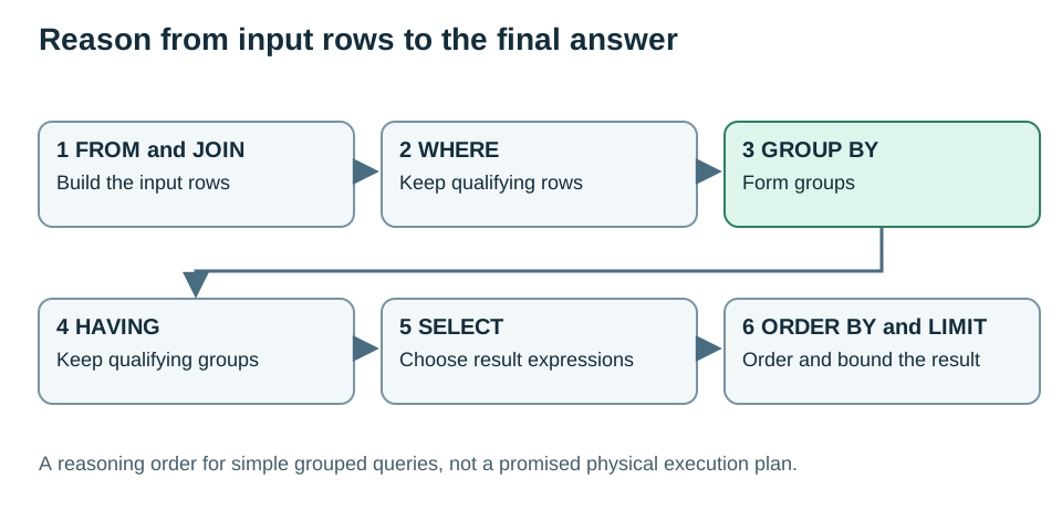
Count completeness honestly
COUNT(*) counts input rows, including rows that contain a null in some columns. COUNT(city) counts only rows with a known city. Their difference is the number with a missing city. COUNT(DISTINCT city) counts different non-null city values. These are three different questions. Use output names that reveal which one was answered.
Most ordinary aggregates ignore null input values. On an empty input, COUNT returns zero while SUM returns NULL. There are no refunds in 2026 in our fixture; that absence produces a null sum rather than a numerical observation. For a display of “total recorded refunds in the period,” COALESCE can intentionally label the absence as zero. Keep the raw interpretation clear in your report. A missing refund feed is not equivalent to a verified period with no refunds.
Averages also require a grain and weighting decision. An average of line amounts answers “typical line,” not “typical order.” An unweighted average of monthly average order values gives each month equal influence, even if the months contain different order counts. For the quarter's average order value, sum the quarter's sales and divide by the quarter's completed orders. Module 12 will make this a verification exercise.
When validating an aggregate, check the groups, totals and exclusions. App plus web completed-order counts should equal the completed-order count before grouping. Reconciliation will not detect every error, especially if both queries share the same wrong filter, so combine it with boundary and hand-worked cases.
Worked example 05 group
App has five completed orders and web has six. HAVING retains both groups. Raising the threshold to six should leave only web.
SELECT channel, COUNT(*) AS completed_orders
FROM aabha_sql.orders WHERE status='completed'
GROUP BY channel HAVING COUNT(*) >= 5 ORDER BY channel;
Expected result from the bundled dataset:
| channel | completed_orders |
|---|---|
| app | 5 |
| web | 6 |
The runnable file is sql/examples/05_group.sql.
Worked example 05 missing
The result separates table coverage from city completeness. Eight customer rows do not imply eight known cities.
SELECT COUNT(*) AS customers, COUNT(city) AS known_cities,
 COUNT(*)-COUNT(city) AS missing_cities FROM aabha_sql.customers;
Expected result from the bundled dataset:
| customers | known_cities | missing_cities |
|---|---|---|
| 8 | 7 | 1 |
The runnable file is sql/examples/05_missing.sql.
Worked example 05 empty
The empty aggregate still returns one summary row. Compare COUNT, the raw SUM and a deliberately labelled display value.
SELECT COUNT(*) AS row_count, SUM(amount) AS raw_sum,
 COALESCE(SUM(amount),0) AS display_sum
FROM aabha_sql.refunds WHERE refund_date >= DATE '2026-01-01';
Expected result from the bundled dataset:
| row_count | raw_sum | display_sum |
|---|---|---|
| 0 | NULL | 0 |
The runnable file is sql/examples/05_empty.sql.
Independent practice
05a
Return each order status and its count as orders. Include every status and sort alphabetically.
Hint: Do not apply the completed-only filter to this question.
05b
Return customer_id and completed_orders for customers with at least two completed orders, sorted by customer_id.
Hint: Filter rows with WHERE, then filter customer groups with HAVING.
Check before moving on
State the grain before and after GROUP BY. Explain why a quarter-wide average order value is not the simple average of three monthly averages.
Module 6 of 13
06 Join relationships and preserve missing matches
Estimated study time: 75–90 minutes. Read, predict, run, explain, then attempt the independent work.
Orders contain customer identifiers, while customer names live in customers. A join lets us combine these facts without storing the name repeatedly on every order. An INNER JOIN produces a row for each pair that satisfies its ON condition. In this relationship, each order's customer_id matches at most one customer because customers.customer_id is a primary key.
Use short table aliases such as o and c, and qualify columns as o.customer_id or c.customer_id. This makes the relationship readable and avoids ambiguity when both inputs contain the same column name. The ON condition compares the intended keys. Matching on names or cities would connect different people who happen to share a label.
Joining orders to customers is many-to-one. It normally preserves the order grain because each order has one matching customer. Joining customers to orders is one-to-many and can create multiple rows for a customer. The SQL text alone does not tell you which grain you wanted; your question does. Write the intended output grain beside the query and check the number of matches.
Use a left join when absence is evidence
The manager asks for every customer's completed-order count, including customers who have not bought. An inner join would omit unmatched customers, so start from customers and LEFT JOIN completed orders. A left join preserves each left-hand row and fills right-hand columns with nulls when no match exists. Gita has no order at all. Hari has a cancelled order but no completed one. Both should appear with zero completed orders.
The status condition belongs inside ON for this question. It controls which order rows may match while retaining every customer. If you write WHERE o.status='completed' after the left join, the synthetic unmatched rows contain a null status and fail the filter. The query effectively loses the customers you intended to keep. Neither placement is universally right; they express different populations.
COUNT(o.order_id) counts real matching orders and ignores the null placeholder. COUNT(*) would count the preserved left row even when no order matched, returning one for a customer who has zero completed orders. This is why you should count a known non-null key from the child table when measuring matches after a left join.
Find the absence rather than hiding it
To find customers with no order of any status, left join all orders and filter WHERE o.order_id IS NULL. You can trust this test because a real order_id is non-null. Testing a nullable descriptive field instead could confuse a matched row with missing detail and a genuinely unmatched row. Module 8 will show NOT EXISTS as another way to express absence.
An inner join's omitted rows can be desirable, but they can also conceal data quality problems. The curated fixture enforces its foreign keys, while the raw intake table deliberately does not. Later we will look for raw customer identifiers that fail to match a known customer. Do not assume that data imported from a CSV has the same guarantees as a constrained table.
A join should be checked in both directions: can a left row disappear, and can it multiply? This module handles disappearance. The next handles multiplication across independent child tables, a frequent source of misleading dashboards and AI-generated SQL.
Worked example 06 join
Each selected order matches one customer, so the four-order result stays at order grain. Customer Asha appears twice because she has two selected orders, not because customers contains duplicate rows.
SELECT o.order_id,c.customer_name,o.channel
FROM aabha_sql.orders AS o JOIN aabha_sql.customers AS c
 ON c.customer_id=o.customer_id
WHERE o.order_id<=1004 ORDER BY o.order_id;
Expected result from the bundled dataset:
| order_id | customer_name | channel |
|---|---|---|
| 1001 | Asha | web |
| 1002 | Ben | app |
| 1003 | Asha | web |
| 1004 | Chen | web |
The runnable file is sql/examples/06_join.sql.
Worked example 06 left
Read the status filter as part of the matching rule. Notice that Gita and Hari survive, and that counting the right-hand order key gives zero for both.
SELECT c.customer_id,c.customer_name,COUNT(o.order_id) AS completed_orders
FROM aabha_sql.customers AS c
LEFT JOIN aabha_sql.orders AS o
 ON o.customer_id=c.customer_id AND o.status='completed'
GROUP BY c.customer_id,c.customer_name ORDER BY c.customer_id;
Expected result from the bundled dataset:
| customer_id | customer_name | completed_orders |
|---|---|---|
| 1 | Asha | 2 |
| 2 | Ben | 3 |
| 3 | Chen | 2 |
| 4 | Divya | 2 |
| 5 | Eren | 1 |
| 6 | Farah | 1 |
| 7 | Gita | 0 |
| 8 | Hari | 0 |
The runnable file is sql/examples/06_left.sql.
Independent practice
06a
For order 1001 join order_items to products and return order_id, line_no, product_name and quantity, sorted by line_no.
Hint: Use product_id for the match; do not substitute the catalogue price for historical unit_price.
06b
Return customer_id and customer_name for customers with no order of any status.
Hint: Start from all customers, preserve unmatched rows, and test the non-null order key for absence.
Check before moving on
Explain the different questions “no orders” and “no completed orders.” Describe exactly why moving the completion filter from ON to WHERE changes the second worked result.
Module 7 of 13
07 Prevent join multiplication and reconcile money
Estimated study time: 75–105 minutes. Read, predict, run, explain, then attempt the independent work.
The manager wants to check sales against successful payments. It is tempting to join order_items directly to payments on order_id and sum both amounts. That query runs, the column names look sensible, and the result can still be wrong. The problem is the combination of two independent one-to-many relationships.
Order 1001 has two lines and two successful payments. Joining only on order_id pairs each line with each payment, producing four rows. The notebook line appears twice and the pen line appears twice. Summing line sales now gives 640 even though the order's line sales are 320. Payments are duplicated in the opposite direction. This is often called join fan-out; the useful mental model is simply “every matching pair becomes a row.”
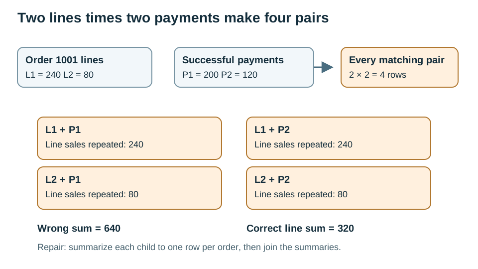
Fix the grain before combining measures
The intended reconciliation grain is one row per order. First aggregate lines to one row per order. Separately aggregate successful payments to one row per order. Then join these two summaries by order_id. Each input now has at most one row for the key, so the combined row contains compatible measures.
The worked repair uses a parenthesized SELECT in FROM. This is a derived table: a query result used as another query's input. Its alias, i or p, lets the outer query refer to its columns. Read and run each inner SELECT independently before considering the join. You already know their SELECT, WHERE and GROUP BY pieces; the new idea is putting their results behind names. Module 8 will introduce WITH as a more readable way to name a chain of intermediate results.
Do not repair this by adding SELECT DISTINCT to the final output. The wrong SUM has already been calculated. SUM(DISTINCT amount) is also unsafe: two real payments can have the same amount, so it may delete legitimate monetary contributions. Deduplicate events using a justified event identifier and source rule, not merely a matching monetary value.
Choose what reconciliation means
Successful payments total the collected amounts in this fixture. Failed attempts must not contribute. Refunds are recorded separately, so comparing successful payments to after-refund net sales would produce expected differences. Here we compare payments to line sales before refunds. Later, net sales subtracts refunds exactly once at order grain. Match the economic definitions before interpreting any difference as a defect.
The inner join in the reference reconciliation returns only orders present in both summaries. It is a useful arithmetic demonstration but is not, on its own, a coverage audit. An order with no successful payment disappears. In our fixture the 11 matched orders are the 11 completed orders; cancelled and pending orders are excluded. For real work, start from the required order population, left join both summaries, and flag missing summaries separately. Never label an absent payment feed as “zero difference.”
Reconciliation is strongest when it combines several independent checks: the expected order population; one output row per order; a hand calculation for a split-payment example; sum of lines versus successful payments; and a separate refund check. A zero grand-total difference can hide a positive error on one order offset by a negative error on another, so examine per-order differences before the final sum.
The deliberately wrong query below is safe to run on synthetic data because it only reads. It is included as a counterexample, not an approved metric. Keep it labelled if you reuse it in teaching.
Worked example 07 fanout
Predict four joined rows from two lines times two payments. The inflated 640 result is deliberately wrong; the true line total is 320.
-- Deliberately incorrect sales metric: two independent child tables multiply rows.
SELECT i.order_id,COUNT(*) AS joined_rows,
 SUM(i.quantity*i.unit_price-i.line_discount) AS inflated_sales
FROM aabha_sql.order_items AS i JOIN aabha_sql.payments AS p ON p.order_id=i.order_id
WHERE i.order_id=1001 AND p.status='succeeded'
GROUP BY i.order_id;
Expected result from the bundled dataset:
| order_id | joined_rows | inflated_sales |
|---|---|---|
| 1001 | 4 | 640.00 |
The runnable file is sql/examples/07_fanout.sql.
Worked example 07 reconcile
Each inner query has order grain. Successful payments and line sales agree for all eleven matched orders. Read the coverage limitation above before using this pattern in production.
SELECT i.order_id,i.line_sales,p.paid_amount,
 i.line_sales-p.paid_amount AS difference
FROM (
 SELECT order_id,SUM(quantity*unit_price-line_discount) AS line_sales
 FROM aabha_sql.order_items GROUP BY order_id
) AS i
JOIN (
 SELECT order_id,SUM(amount) AS paid_amount
 FROM aabha_sql.payments WHERE status='succeeded' GROUP BY order_id
) AS p ON p.order_id=i.order_id
ORDER BY i.order_id;
Expected result from the bundled dataset:
| order_id | line_sales | paid_amount | difference |
|---|---|---|---|
| 1001 | 320.00 | 320.00 | 0.00 |
| 1002 | 800.00 | 800.00 | 0.00 |
| 1004 | 520.00 | 520.00 | 0.00 |
| 1005 | 450.00 | 450.00 | 0.00 |
| 1006 | 840.00 | 840.00 | 0.00 |
| 1008 | 360.00 | 360.00 | 0.00 |
| 1009 | 750.00 | 750.00 | 0.00 |
| 1010 | 920.00 | 920.00 | 0.00 |
| 1011 | 200.00 | 200.00 | 0.00 |
| 1012 | 450.00 | 450.00 | 0.00 |
| 1014 | 250.00 | 250.00 | 0.00 |
The runnable file is sql/examples/07_reconcile.sql.
Independent practice
07a
Join items and successful payments for order 1006 directly. Return order_id, joined_rows and inflated_payments. Explain why the payment sum doubles.
Hint: Ignore the failed attempt; two lines still pair with two successful payments.
07b
Repair the order 1006 reconciliation using two grouped derived tables. Return order_id, line_sales and paid_amount.
Hint: Each derived table must output one row for order 1006 before the join.
Check before moving on
You can explain a four-row join on paper, identify each measure’s original grain, and justify why monetary DISTINCT is not a safe deduplication policy.
Module 8 of 13
08 Build readable analysis with subqueries and CTEs
Estimated study time: 75–105 minutes. Read, predict, run, explain, then attempt the independent work.
A useful analysis often needs an answer from an earlier analysis. To find catalogue products above the average price, calculate the average first and compare each price against it. A scalar subquery returns one value, such as AVG(list_price). The outer WHERE can then use that value like another expression. If a scalar subquery returns multiple rows, PostgreSQL raises an error; it cannot guess which one you meant.
A different need is to test whether a relationship exists. EXISTS is true when its subquery finds at least one row. NOT EXISTS is true when it finds none. In the customer example, the subquery refers to c.customer_id from the outer query; this is a correlated subquery. Read it as “for this customer, is there any completed order?” The result is still one row per outer customer, rather than one row per matching order.
NOT EXISTS also avoids a subtle trap with NOT IN. If a NOT IN subquery contains a null, a nonmatching comparison can become unknown and be removed by WHERE. Use NOT EXISTS when the question is the absence of a matching relationship, and still be explicit about how null keys should be treated. Curated customer keys here are non-null.
Give intermediate results meaningful names
WITH introduces common table expressions, or CTEs. A CTE is a named query result available within the statement. It is not automatically a permanent table, and it is not a guarantee that the database materializes a physical copy. Use it first to make reasoning and testing clearer, not as a magic performance improvement.
The net-sales example has three stages. line_totals produces one row per order from item lines. refund_totals produces one row per order from refunds recorded before the reporting cutoff. order_net joins those summaries to completed orders inside the quarter and computes after-refund net sales. The final SELECT inspects individual order values. Each name says what the rows mean; each stage has an explicit key.
A left join is required for refunds because many completed orders have no refund record. Here COALESCE(refunded,0) has a justified meaning: within this complete synthetic refund ledger, no matching refund means no recorded refund amount. If a production ledger were incomplete, zero would be an assumption needing validation. line_totals uses an inner join because the fixture contains lines for every order; a real audit must check missing-line coverage separately.
Keep the reporting clock visible
The refund cutoff is before 1 April, and order inclusion uses the same quarter-end boundary. Refunds are assigned to the original order month. This reports the quarter's orders net of refunds known by the cutoff; it is different from a cash-flow report grouped by refund date. A late refund after 1 April would not belong in this particular as-of report.
We have current order status, not a status-history table. For this teaching fixture we assume that each stored completion was known on the order date. That assumption is deliberately stated because an actual historical report cannot infer past status from a current snapshot. Module 11 will make the same limitation important for AI features.
Build a CTE pipeline one stage at a time. Run the first stage's query alone, inspect keys and totals, then add the second. If the final result is wrong, inspect the earliest stage where an expected invariant fails. This approach is faster and more reliable than editing a long query randomly or asking a model to rewrite it without a diagnosis.
Worked example 08 scalar
The product-price average is a single scalar. The bag and guide exceed it. This uses catalogue prices because the question is about the current catalogue.
SELECT product_id,product_name,list_price FROM aabha_sql.products
WHERE list_price > (SELECT AVG(list_price) FROM aabha_sql.products)
ORDER BY list_price DESC,product_id;
Expected result from the bundled dataset:
| product_id | product_name | list_price |
|---|---|---|
| 104 | Bag | 800.00 |
| 105 | Guide | 500.00 |
The runnable file is sql/examples/08_scalar.sql.
Worked example 08 exists
The existence check does not multiply customers with several orders. It finds Gita and Hari because neither has a completed order.
SELECT c.customer_id,c.customer_name FROM aabha_sql.customers AS c
WHERE NOT EXISTS (SELECT 1 FROM aabha_sql.orders AS o
 WHERE o.customer_id=c.customer_id AND o.status='completed')
ORDER BY c.customer_id;
Expected result from the bundled dataset:
| customer_id | customer_name |
|---|---|
| 7 | Gita |
| 8 | Hari |
The runnable file is sql/examples/08_exists.sql.
Worked example 08 cte
Read from line_totals through order_net. Order 1005 has two refund records totalling 75, so 450 of line sales becomes 375 of net sales.
WITH line_totals AS (
 SELECT order_id,SUM(quantity*unit_price-line_discount) AS line_sales
 FROM aabha_sql.order_items GROUP BY order_id
), refund_totals AS (
 SELECT order_id,SUM(amount) AS refunded
 FROM aabha_sql.refunds WHERE refund_date < DATE '2025-04-01' GROUP BY order_id
), order_net AS (
 SELECT o.order_id,o.customer_id,o.order_date,o.channel,
 l.line_sales,COALESCE(r.refunded,0) AS refunded,
 l.line_sales-COALESCE(r.refunded,0) AS net_sales
 FROM aabha_sql.orders AS o
 JOIN line_totals AS l ON l.order_id=o.order_id
 LEFT JOIN refund_totals AS r ON r.order_id=o.order_id
 WHERE o.status='completed' AND o.order_date >= DATE '2025-01-01'
   AND o.order_date < DATE '2025-04-01'
)
SELECT order_id,line_sales,refunded,net_sales FROM order_net ORDER BY order_id;
Expected result from the bundled dataset:
| order_id | line_sales | refunded | net_sales |
|---|---|---|---|
| 1001 | 320.00 | 20.00 | 300.00 |
| 1002 | 800.00 | 0 | 800.00 |
| 1004 | 520.00 | 0 | 520.00 |
| 1005 | 450.00 | 75.00 | 375.00 |
| 1006 | 840.00 | 0 | 840.00 |
| 1008 | 360.00 | 0 | 360.00 |
| 1009 | 750.00 | 0 | 750.00 |
| 1010 | 920.00 | 120.00 | 800.00 |
| 1011 | 200.00 | 0 | 200.00 |
| 1012 | 450.00 | 0 | 450.00 |
| 1014 | 250.00 | 0 | 250.00 |
The runnable file is sql/examples/08_cte.sql.
Independent practice
08a
Return customer_id and customer_name for customers who have at least one refund on any order. Return each customer once.
Hint: Use EXISTS with the orders-to-refunds relationship inside it.
08b
Starting from the order_net CTE pattern, return channel and total net_sales for the quarter, ordered by channel.
Hint: Keep the cutoff and refund rules unchanged; only the final aggregation changes.
Check before moving on
You can state the grain and key of each CTE, explain why refunds use a left join, and distinguish an as-of sales report from refund-date cash flow.
Module 9 of 13
09 Compare rows with window functions
Estimated study time: 75–105 minutes. Read, predict, run, explain, then attempt the independent work.
A monthly total compresses orders into one row per month. The manager now wants to keep those month rows while adding a running total and the preceding month's sales. A window function performs a calculation across related result rows without collapsing them. The presence of OVER distinguishes it from an ordinary grouped aggregate.
Start by producing the monthly totals at the correct grain. In the worked query, GROUP BY 1 refers to the first expression in its SELECT list, the month key. This positional shorthand is valid PostgreSQL, but repeating the explicit month expression is often clearer when a query is likely to be edited. Then SUM(net_sales) OVER (...) can add a cumulative figure beside each month. The window's ORDER BY determines the sequence used in that calculation. The final ORDER BY controls presentation. These are separate roles; one should not be assumed to imply the other.
ROWS BETWEEN UNBOUNDED PRECEDING AND CURRENT ROW explicitly defines the cumulative frame: begin with the first ordered row and end at this row. When ordering contains ties, PostgreSQL's default frame can include peers with the same ordering value. An explicit ROWS frame plus a deterministic ordering removes surprises for a row-by-row cumulative measure. Here the monthly aggregation makes the month key unique, which also makes the sequence clear.
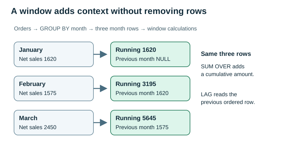
Compare with a previous result row
LAG(net_sales) retrieves the preceding row's amount in the window order. The first row has no predecessor, so the result is null. That is a boundary fact, not a zero-sales month. The difference between current and prior sales gives an absolute change. Dividing that difference by the prior value gives a relative change, with NULLIF protecting a zero denominator.
LAG means “previous row,” not necessarily “previous calendar month.” Our fixture contains January, February and March. If February were absent, March's previous row would be January. A complete calendar series and an agreed missing-month policy are needed before claiming true month-over-month change on sparse data. Do not silently replace a missing month with zero if the source might simply be incomplete.
Rank customers with a tie policy
ROW_NUMBER assigns different sequential positions even when scores tie; add customer_id to make ties deterministic. DENSE_RANK assigns the same rank to equal scores and leaves no gaps after a tie. RANK also shares a rank but leaves gaps. Choose the function that matches the question. “Exactly two rows for display” differs from “everyone tied within the top two ranks.”
The worked query uses net_sales alone inside DENSE_RANK so equal amounts would share a rank. It uses net_sales and customer_id inside ROW_NUMBER to guarantee a stable display order. Adding the identifier to the ranking expression would accidentally make every row distinct and defeat the business tie policy.
A window expression cannot be filtered by WHERE at the same query level because the window calculation occurs later in the logical reasoning sequence. To keep only the top two positions, calculate positions in a CTE and filter that CTE in an outer SELECT. You already know this staged pattern from module 8; now the intermediate result includes a window value.
Use PARTITION BY inside OVER when the comparison should restart for each group, such as a separate ranking within every channel. Without it, the whole input result is one partition. The grouped aggregate, the partition and the final ordering answer different questions. Draw the rows and label each boundary before choosing syntax.
Worked example 09 running
Three monthly rows remain three rows. The running total reaches 5645 in March, which reconciles to the full-quarter net total.
WITH line_totals AS (
 SELECT order_id,SUM(quantity*unit_price-line_discount) AS line_sales
 FROM aabha_sql.order_items GROUP BY order_id
), refund_totals AS (
 SELECT order_id,SUM(amount) AS refunded
 FROM aabha_sql.refunds WHERE refund_date < DATE '2025-04-01' GROUP BY order_id
), order_net AS (
 SELECT o.order_id,o.customer_id,o.order_date,o.channel,
 l.line_sales,COALESCE(r.refunded,0) AS refunded,
 l.line_sales-COALESCE(r.refunded,0) AS net_sales
 FROM aabha_sql.orders AS o
 JOIN line_totals AS l ON l.order_id=o.order_id
 LEFT JOIN refund_totals AS r ON r.order_id=o.order_id
 WHERE o.status='completed' AND o.order_date >= DATE '2025-01-01'
   AND o.order_date < DATE '2025-04-01'
), monthly AS (
 SELECT date_trunc('month',order_date)::date AS month,SUM(net_sales) AS net_sales
 FROM order_net GROUP BY 1
)
SELECT month::text AS month,net_sales,
 SUM(net_sales) OVER (ORDER BY month ROWS BETWEEN UNBOUNDED PRECEDING AND CURRENT ROW) AS running_sales,
 LAG(net_sales) OVER (ORDER BY month) AS previous_month_sales
FROM monthly ORDER BY month;
Expected result from the bundled dataset:
| month | net_sales | running_sales | previous_month_sales |
|---|---|---|---|
| 2025-01-01 | 1620.00 | 1620.00 | NULL |
| 2025-02-01 | 1575.00 | 3195.00 | 1620.00 |
| 2025-03-01 | 2450.00 | 5645.00 | 1575.00 |
The runnable file is sql/examples/09_running.sql.
Worked example 09 rank
The fixture has no sales ties, so the two position columns agree. The validator includes a separate tied-score case to check the intended distinction.
WITH line_totals AS (
 SELECT order_id,SUM(quantity*unit_price-line_discount) AS line_sales
 FROM aabha_sql.order_items GROUP BY order_id
), refund_totals AS (
 SELECT order_id,SUM(amount) AS refunded
 FROM aabha_sql.refunds WHERE refund_date < DATE '2025-04-01' GROUP BY order_id
), order_net AS (
 SELECT o.order_id,o.customer_id,o.order_date,o.channel,
 l.line_sales,COALESCE(r.refunded,0) AS refunded,
 l.line_sales-COALESCE(r.refunded,0) AS net_sales
 FROM aabha_sql.orders AS o
 JOIN line_totals AS l ON l.order_id=o.order_id
 LEFT JOIN refund_totals AS r ON r.order_id=o.order_id
 WHERE o.status='completed' AND o.order_date >= DATE '2025-01-01'
   AND o.order_date < DATE '2025-04-01'
), customer_sales AS (
 SELECT customer_id,SUM(net_sales) AS net_sales FROM order_net GROUP BY customer_id
)
SELECT customer_id,net_sales,DENSE_RANK() OVER (ORDER BY net_sales DESC) AS sales_rank,
 ROW_NUMBER() OVER (ORDER BY net_sales DESC,customer_id) AS display_position
FROM customer_sales ORDER BY display_position;
Expected result from the bundled dataset:
| customer_id | net_sales | sales_rank | display_position |
|---|---|---|---|
| 2 | 1890.00 | 1 | 1 |
| 3 | 1270.00 | 2 | 2 |
| 1 | 1100.00 | 3 | 3 |
| 4 | 575.00 | 4 | 4 |
| 5 | 450.00 | 5 | 5 |
| 6 | 360.00 | 6 | 6 |
The runnable file is sql/examples/09_rank.sql.
Independent practice
09a
Return exactly the top two purchasing customers with customer_id, net_sales and position. Break amount ties with customer_id.
Hint: Calculate ROW_NUMBER in a CTE, then apply the position filter outside it.
09b
Return month, absolute_change and percent_change in net sales from the preceding month. Keep the first month’s change null and round percentage change to two decimals.
Hint: Calculate LAG in one stage and the differences in the next. A missing or zero denominator must not become a claimed zero percent change.
Check before moving on
Explain why window SUM retains rows, why a deterministic tie-breaker matters, and why LAG alone does not fill gaps in a calendar.
Module 10 of 13
10 Audit quality before trusting the result
Estimated study time: 75–105 minutes. Read, predict, run, explain, then attempt the independent work.
So far, curated tables have had valid keys and constrained values. Real data often arrives in a raw area before those guarantees exist. Our raw_orders table deliberately contains repeated source identifiers, a negative amount, an unknown customer, an impossible date, an unexpected status and missing fields. Your task is to identify and document these defects, not make them disappear until the output looks tidy.
A primary key on batch_row only identifies the received row. It does not make source_order_id unique. The duplicate query groups by the business identifier and finds two versions of 9001. They arrived at different times. This fixture's policy is to prefer the latest loaded_at value, with batch_row as a deterministic tie-breaker. That is a source-specific policy, not a universal truth about duplicates.
Separate normalization from invention
LOWER(TRIM(status_text)) removes surrounding whitespace and normalizes letter case. It converts ' Completed ' and 'COMPLETED' into 'completed'. It does not turn 'complete' into 'completed'; that mapping needs an approved meaning, because an unfamiliar source value might have a different definition. The audit flags it rather than guessing.
A missing amount differs from a negative amount. Both fail this fixture's acceptance rule, but they require different investigation. Similarly, customer_id 99 is an unknown reference while a null customer_id is absent altogether. Keep reason columns separate so that one row can show several problems at once. A single first-error label can hide additional defects.
Dates arrive as text in the raw table. A string shaped like YYYY-MM-DD can still be impossible, such as 2025-02-30. PostgreSQL's pg_input_is_valid checks whether the text can be read as the specified type without forcing a failing cast. This function requires PostgreSQL 16 or later, and this package is tested on the bundled PostgreSQL 18-based runtime. It validates PostgreSQL date input, not a strict organizational ISO-only policy. Add an explicit format rule if that is part of your contract.
Deduplication is not validation
The dedupe example chooses one latest version per source_order_id using ROW_NUMBER. Its output still contains the negative amount, bad customer and invalid date. Fewer rows do not mean cleaner rows. In the independent task, choose the latest version first and then apply the acceptance checks. If the latest version is invalid, quarantine that identifier for review rather than silently falling back to an older record. A different policy would need an explicit business decision.
Do not mutate raw evidence during an audit. Preserve the received rows, record the rule version, and produce a separate accepted result and issue report. This makes it possible to explain why a record was excluded, investigate a supplier correction and reproduce the report. Excluding bad rows also changes coverage; a report should name how many source entities were accepted and what remains unresolved.
Quality is broader than row validity. Ask whether the file is fresh, whether the expected time range is complete, whether monetary units agree, whether an identifier is stable, and whether the data represents the population your question concerns. A perfectly valid table from last month cannot answer today's operational question. Our small synthetic file is intentionally complete for its stated teaching period, not evidence about a real business.
The curated schema's constraints and the raw audit serve different stages. Constraints stop certain invalid states from entering a curated table. Read-only audit queries explain what was wrong before that boundary. Neither proves that a name, amount or event is factually true in the outside world.
Worked example 10 duplicates
There are eight received rows but only seven source identifiers. The repeated identifier is not automatically an extra order.
SELECT source_order_id,COUNT(*) AS versions
FROM aabha_sql.raw_orders GROUP BY source_order_id HAVING COUNT(*)>1 ORDER BY source_order_id;
Expected result from the bundled dataset:
| source_order_id | versions |
|---|---|
| 9001 | 2 |
The runnable file is sql/examples/10_duplicates.sql.
Worked example 10 audit
Inspect every reason column. Raw row 7 has both a missing customer and a missing amount, while row 5 has an impossible calendar date.
SELECT r.batch_row,r.source_order_id,
 CASE WHEN r.customer_id IS NULL THEN 'missing_customer'
      WHEN c.customer_id IS NULL THEN 'unknown_customer' ELSE 'ok' END AS customer_check,
 CASE WHEN r.amount IS NULL THEN 'missing_amount'
      WHEN r.amount<0 THEN 'negative_amount' ELSE 'ok' END AS amount_check,
 CASE WHEN lower(trim(r.status_text)) IN ('completed','pending','cancelled') THEN 'ok'
      ELSE 'unknown_status' END AS status_check,
 CASE WHEN r.order_date_text IS NOT NULL AND pg_input_is_valid(r.order_date_text,'date')
      THEN 'ok' ELSE 'invalid_date' END AS date_check
FROM aabha_sql.raw_orders AS r LEFT JOIN aabha_sql.customers AS c
 ON c.customer_id=r.customer_id ORDER BY r.batch_row;
Expected result from the bundled dataset:
| batch_row | source_order_id | customer_check | amount_check | status_check | date_check |
|---|---|---|---|---|---|
| 1 | 9001 | ok | ok | ok | ok |
| 2 | 9001 | ok | ok | ok | ok |
| 3 | 9002 | ok | negative_amount | ok | ok |
| 4 | 9003 | unknown_customer | ok | ok | ok |
| 5 | 9004 | ok | ok | ok | invalid_date |
| 6 | 9005 | ok | ok | unknown_status | ok |
| 7 | 9006 | missing_customer | missing_amount | ok | ok |
| 8 | 9007 | ok | ok | ok | ok |
The runnable file is sql/examples/10_audit.sql.
Worked example 10 dedupe
Row 2 wins over row 1 because it arrived later. The remaining defects are intentionally still present, demonstrating why deduplication and validity are separate steps.
WITH ranked AS (
 SELECT batch_row,source_order_id,lower(trim(status_text)) AS status,
 ROW_NUMBER() OVER (PARTITION BY source_order_id ORDER BY loaded_at DESC,batch_row DESC) AS position
 FROM aabha_sql.raw_orders
)
SELECT batch_row,source_order_id,status FROM ranked WHERE position=1 ORDER BY source_order_id;
Expected result from the bundled dataset:
| batch_row | source_order_id | status |
|---|---|---|
| 2 | 9001 | completed |
| 3 | 9002 | completed |
| 4 | 9003 | completed |
| 5 | 9004 | completed |
| 6 | 9005 | complete |
| 7 | 9006 | pending |
| 8 | 9007 | completed |
The runnable file is sql/examples/10_dedupe.sql.
Independent practice
10a
Return batch_row and customer_id for raw rows with a non-null customer identifier that is absent from customers.
Hint: Distinguish unknown identifiers from missing identifiers; use a left join and an explicit non-null source test.
10b
Choose the latest version per source_order_id, then accept only non-null source_order_id values, known customers, non-null nonnegative amounts, recognized normalized statuses and valid non-null dates. Return batch_row, source_order_id, normalized status and amount.
Hint: Use the ranked CTE from the example. In WHERE, a null amount does not satisfy amount >= 0. Do not cast date text before validating it.
Check before moving on
Explain why only two raw rows survive the acceptance policy, why raw evidence should be preserved, and which quality risks are not covered by these row-level checks.
Module 11 of 13
11 Prepare AI features without future leakage
Estimated study time: 75–105 minutes. Read, predict, run, explain, then attempt the independent work.
SQL often supplies a machine-learning dataset. Before choosing a model, decide what one training row represents and when the prediction would have been made. Here the illustrative question is: among customers already registered before 1 March 2025, who will place a completed order during March? One row represents an eligible customer at the 1 March cutoff.
A feature is information available at that prediction time. A label is the future outcome we later observe. We will use January and February completed-order counts, sales before refunds and recency as features. The label is whether the customer buys during March. The code that constructs those two pieces must keep their time boundaries separate.
The feature query starts with eligible_orders, selecting only completed orders dated before 1 March and no earlier than 1 January. It aggregates lines to order grain, then orders to customer grain. A final left join begins from the eligible customer population, retaining customers who have no qualifying orders. Eren is registered before the cutoff but has only a pending February order, so the feature row has zero completed orders and zero sales.
Recency is the days from the last qualifying order to the cutoff. Eren has no such order, so recency is null. Replacing it with zero would incorrectly mean “ordered on the cutoff day.” A downstream model may need an imputation rule and a missingness indicator, but that is a separate modeling decision learned on training data. The SQL extraction should preserve the meaning first.
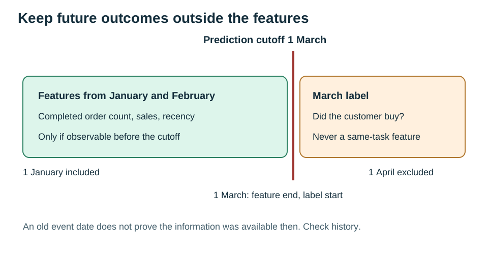
A date filter alone cannot recover history
The fixture assumes that a stored completed status was known on the order date and that relevant records arrived without delay. That is a simplifying teaching assumption. A real database often stores current status only. If an order was pending on 28 February but completed on 3 March, using today's completed status can leak future information even when order_date is before 1 March. A genuine historical feature table needs status-effective times or trustworthy as-of snapshots, plus source availability timestamps when late arrival matters.
The same concern applies to refunds, customer attributes and corrected records. Our chosen sales feature deliberately uses line sales before refunds and is named accordingly. It is not the quarter's net-sales metric from the capstone. A production net-spend feature would need refunds observable before the prediction cutoff, not all refunds known today.
Keep population and outcome definitions aligned
The label query uses the same eligible customers as the features, then searches only March completed orders. Customers who registered on or after 1 March are excluded from both sides. Gita, registered exactly on 1 March, is not silently added because she exists in today's customer table. Join features to labels on customer_id and verify that both sides have exactly one row for each eligible key.
Do not feed bought_in_march, March order counts or March revenue back into the feature columns. Those describe the outcome you are trying to predict. Also avoid using identifiers as unexplained predictive signals, including unnecessary names, or exporting personal details simply because they are available. This exercise needs customer_id only for alignment; it is not automatically a useful model input.
The six-row fixture teaches extraction mechanics. It is far too small to establish model quality, fairness or a business-ready recommendation. A real project needs an appropriate population, time-based evaluation, leakage checks and a documented data-access basis. SQL correctness is necessary for that work, but it does not make the learning problem valid by itself.
Worked example 11 features
Follow the two aggregation stages and then the population-preserving join. The expected six rows include Eren with null recency. Farah’s February 28 order is one day before the cutoff.
WITH eligible_orders AS (
 SELECT o.order_id,o.customer_id,o.order_date,
 SUM(i.quantity*i.unit_price-i.line_discount) AS sales_before_refunds
 FROM aabha_sql.orders AS o JOIN aabha_sql.order_items AS i ON i.order_id=o.order_id
 WHERE o.status='completed' AND o.order_date >= DATE '2025-01-01'
   AND o.order_date < DATE '2025-03-01'
 GROUP BY o.order_id,o.customer_id,o.order_date
), customer_features AS (
 SELECT customer_id,COUNT(*) AS completed_orders,
 SUM(sales_before_refunds) AS sales_before_refunds,MAX(order_date) AS last_order_date
 FROM eligible_orders GROUP BY customer_id
)
SELECT c.customer_id,COALESCE(f.completed_orders,0) AS completed_orders,
 COALESCE(f.sales_before_refunds,0) AS sales_before_refunds,
 DATE '2025-03-01'-f.last_order_date AS recency_days
FROM aabha_sql.customers AS c LEFT JOIN customer_features AS f ON f.customer_id=c.customer_id
WHERE c.signup_date < DATE '2025-03-01'
ORDER BY c.customer_id;
Expected result from the bundled dataset:
| customer_id | completed_orders | sales_before_refunds | recency_days |
|---|---|---|---|
| 1 | 1 | 320.00 | 55 |
| 2 | 2 | 1640.00 | 15 |
| 3 | 1 | 520.00 | 29 |
| 4 | 1 | 450.00 | 28 |
| 5 | 0 | 0 | NULL |
| 6 | 1 | 360.00 | 1 |
The runnable file is sql/examples/11_features.sql.
Worked example 11 labels
The March outcome is separate. It must never be used as an input feature for the same March prediction.
SELECT c.customer_id,
 CASE WHEN EXISTS (SELECT 1 FROM aabha_sql.orders AS o WHERE o.customer_id=c.customer_id
 AND o.status='completed' AND o.order_date>=DATE '2025-03-01'
 AND o.order_date<DATE '2025-04-01') THEN 1 ELSE 0 END AS bought_in_march
FROM aabha_sql.customers AS c WHERE c.signup_date<DATE '2025-03-01' ORDER BY c.customer_id;
Expected result from the bundled dataset:
| customer_id | bought_in_march |
|---|---|
| 1 | 1 |
| 2 | 1 |
| 3 | 1 |
| 4 | 1 |
| 5 | 1 |
| 6 | 0 |
The runnable file is sql/examples/11_labels.sql.
Independent practice
11a
Count customers eligible for a prediction at 1 March using the stated registration rule. Name the result eligible_customers.
Hint: A customer registered exactly on the cutoff is outside the before-cutoff population.
11b
Wrap the supplied feature query in a features CTE and compare its row count with COUNT(DISTINCT customer_id). Return rows and distinct_customers. Then write one paragraph naming two real-world leakage risks this static fixture cannot resolve.
Hint: Remove the inner query’s final semicolon before enclosing it in a CTE. Matching counts check uniqueness, not time validity.
Check before moving on
You can identify the prediction time, feature window, label window, population and observation-history assumption. Do not claim a production-ready training dataset from this fixture.
Module 12 of 13
12 Use AI as a checked SQL assistant
Estimated study time: 75–90 minutes. Read, predict, run, explain, then attempt the independent work.
An AI assistant can explain an error, suggest a query skeleton or propose edge cases. It can also invent columns, choose an unintended definition of revenue or produce a join that multiplies money. The safest working relationship is to let the model propose a draft while you own the metric, access boundary and verification evidence.
Begin with a short data contract. Give the dialect, allowed tables and columns, primary and foreign keys, table grains, date boundaries and business definitions. State the desired output grain and inclusion rules. Ask the assistant to list assumptions and uncertain points before writing SQL. Supply only approved metadata and synthetic examples; a useful query draft rarely needs raw customer names, credentials or full production records.
A prompt that makes review possible
Use the following prompt with an AI tool you are already allowed to use, or complete the review manually. No AI account or paid service is required to finish the course.
“Draft a read-only PostgreSQL query using the synthetic Aabha schema. Return one row per month for completed orders dated from 2025-01-01 inclusive to 2025-04-01 exclusive. Line sales are quantity times historical unit_price minus the total line_discount. Subtract refunds recorded before 2025-04-01 and assign them to the original order month. Aggregate independent child tables before joining. Return order count, buyer count, before-refund sales, refunds, net sales and net average order value. Explain the grain of every intermediate result, identify assumptions, and propose tests. Do not invent columns or execute anything.”
The prompt helps but is not a security control. A model's statement that a query is safe or correct is a claim to test. Compare every identifier with the schema. Read every statement, including CTEs. A statement beginning WITH can contain modifying operations; a SELECT can call functions with side effects or reveal data. Do not use keyword matching as your only defense.
Verify meaning as well as syntax
First, test in the isolated synthetic lab. Check one-row-per-order uniqueness before the monthly grouping, reconcile before-refund sales minus refunds to net sales, and verify the known boundary orders. Use the split-payment case to catch fan-out. Compare a hand-calculated order with the result. Check empty inputs, missing values and a zero denominator. If the model changes its query, rerun the tests instead of assuming the change is cosmetic.
Then review the business interpretation. Does the average divide by orders or lines? Are failed payment attempts excluded? Are buyers counted distinctly within each month rather than summed as if unique across the whole quarter? Does the refund cutoff match the report? A query can parse and return the expected number of columns while answering the wrong question.
Read-only is layered protection
The supplied runner opens a fresh in-memory database and starts a READ ONLY transaction for analysis, with a five-second statement timeout. Read-only transactions block ordinary changes to persistent tables; they are not a complete sandbox or a defense against data disclosure, expensive queries or all side effects. An untrusted script could try to end a transaction. Therefore the runner is for your reviewed practice queries, not for safely executing arbitrary hostile SQL.
In real systems, use a dedicated least-privilege account approved by the database owner, restricted views where appropriate, access auditing, query limits and reviewed parameterized application queries. Keep credentials out of prompts. These operational controls must be arranged with the system owner; this course does not configure production access. Values supplied by application users should be bound as parameters, rather than concatenated into SQL text. Identifiers require a separate controlled selection policy.
EXPLAIN shows an estimated execution plan without running the analyzed SELECT. It can reveal a scan or join shape, but an estimated plan is not proof of speed or correctness. EXPLAIN ANALYZE actually executes the statement, which matters for costly or modifying operations. Our tiny fixture's plan and timing cannot establish production performance.
Keep a short review record: the question, schema version, query, assumptions, test evidence and unresolved limitations. This is more useful than keeping only a screenshot of a plausible result.
Worked example 12 verify
The query checks order-grain uniqueness and three monetary totals. Its 5860 minus 215 equals 5645, but the independent boundary and coverage checks remain necessary.
WITH line_totals AS (
 SELECT order_id,SUM(quantity*unit_price-line_discount) AS line_sales
 FROM aabha_sql.order_items GROUP BY order_id
), refund_totals AS (
 SELECT order_id,SUM(amount) AS refunded
 FROM aabha_sql.refunds WHERE refund_date < DATE '2025-04-01' GROUP BY order_id
), order_net AS (
 SELECT o.order_id,o.customer_id,o.order_date,o.channel,
 l.line_sales,COALESCE(r.refunded,0) AS refunded,
 l.line_sales-COALESCE(r.refunded,0) AS net_sales
 FROM aabha_sql.orders AS o
 JOIN line_totals AS l ON l.order_id=o.order_id
 LEFT JOIN refund_totals AS r ON r.order_id=o.order_id
 WHERE o.status='completed' AND o.order_date >= DATE '2025-01-01'
   AND o.order_date < DATE '2025-04-01'
)
SELECT COUNT(*) AS rows,COUNT(DISTINCT order_id) AS distinct_orders,
 SUM(line_sales) AS sales_before_refunds,SUM(refunded) AS refunds,SUM(net_sales) AS net_sales
FROM order_net;
Expected result from the bundled dataset:
| rows | distinct_orders | sales_before_refunds | refunds | net_sales |
|---|---|---|---|---|
| 11 | 11 | 5860.00 | 215.00 | 5645.00 |
The runnable file is sql/examples/12_verify.sql.
Worked example 12 explain
Inspect the plan shape rather than memorizing the exact cost numbers. The validator checks that a plan is returned; costs may differ across PostgreSQL builds or statistics.
EXPLAIN SELECT order_id FROM aabha_sql.orders
WHERE order_date >= DATE '2025-03-01' AND order_date < DATE '2025-04-01';
Expected result from the bundled dataset:
| QUERY PLAN |
|---|
| Seq Scan on orders (cost=0.00..21.70 rows=4 width=4) |
| Filter: ((order_date >= '2025-03-01'::date) AND (order_date < '2025-04-01'::date)) |
The runnable file is sql/examples/12_explain.sql.
Independent practice
12a
An AI draft starts from customers and left joins orders, then filters WHERE o.status = 'completed' and counts COUNT(*). Repair the report to keep all customers with correct completed-order counts. Explain both errors.
Hint: The quoted text describes a flawed draft, not executable SQL. Revisit where the completion condition belongs and which key should be counted.
12b
Compute full-quarter net_average_order_value from order_net. Return net_sales, completed_orders and the rounded average. Explain why an average of the three monthly averages is not equivalent.
Hint: Use the full-quarter order denominator. No external AI tool is needed.
Check before moving on
You can reject a plausible SQL draft for a concrete reason, reproduce the failure on synthetic data, and name safety controls beyond a READ ONLY transaction.
Module 13 of 13
13 Deliver a checked analysis capstone
Estimated study time: 120–180 minutes. Read, predict, run, explain, then attempt the independent work.
You are the analyst for the fictional retailer. The manager needs a concise quarter review before deciding what to investigate next. Your job is to produce reproducible SQL evidence and a cautious explanation. The dataset does not contain marketing spend, profit, inventory, website traffic or an experiment, so your report cannot attribute changes to a campaign or explain causal drivers.
Start by writing a metric contract in your own words. Use completed orders placed from 1 January 2025 inclusive to 1 April exclusive. Historical line prices and total line discounts define before-refund sales. Subtract refunds recorded before 1 April, assigning each refund to the original order month. The population includes all eight registered customers when reporting customer contribution, even if their completed-order count is zero. The source is a fixed synthetic snapshot.
Build the report in an inspectable sequence
First verify the source counts and keys. Next build a one-row-per-order intermediate result using independent line and refund summaries. Check that the 11 completed orders remain 11 distinct order identifiers. Reconcile the line-sales total, refunds and net sales. Only then aggregate to months and customer contribution. This sequence lets a reviewer locate a wrong result rather than inspect a single opaque query.
Your monthly output must contain month, completed_orders, buying_customers, sales_before_refunds, refunds, net_sales and net_average_order_value. Count buyers distinctly inside each month. A customer can buy in several months, so adding monthly buyer counts does not yield quarter-unique customers. The customer output must include all customers with identifier, synthetic name, completed-order count and net sales, sorted by sales descending and identifier as a tie-breaker.
The worked report below is a review target. For an assessed attempt, finish your own SQL and written findings before opening the separate solutions. If you are self-studying, use the checkpoint totals to diagnose a mismatch, but explain the cause of the mismatch rather than copying the answer. A correct number with an incorrect method will fail when the data changes.
Read the pattern without inventing a cause
The monthly net sales are 1620, 1575 and 2450. March has more completed orders than February, but a lower net average order value. Those two observations can coexist: total sales increased while the average value per completed order decreased. The data supports describing that arithmetic pattern; it does not establish why customers behaved differently.
Ben contributes the most quarter net sales in this fixture. That is a descriptive ranking of six purchasing customers, not evidence for targeting or treating real people differently. Gita and Hari remain in the customer output with zero completed sales for different reasons. Preserve those distinctions when proposing follow-up questions.
A useful summary says what changed, how the measure was defined, and what evidence is missing. For example, ask whether the order mix changed, but do not claim that a specific campaign caused the increase without campaign data and a suitable analysis. The best next question is one the current evidence motivates and the next data collection could actually answer.
Submit a reproducible package
Submit your two SQL queries, a brief metric contract, an audit note with source counts and reconciliation checks, and a 150–250 word manager summary. Include one chart or a simple monthly table, with INR units and the as-of cutoff. Also include your module 11 feature table and a short leakage-risk note so the analysis-to-AI connection remains visible.
Use the rubric in ASSESSMENT.md. Correct grain, coverage, date boundaries and safety are required for a pass; attractive charts cannot compensate for duplicated money. The reference implementation and explanation are in SOLUTIONS.md and sql/solutions. No certificate, external credit or learner progress is automatically issued by this package.
Worked example 13 monthly
Use this as a review target after an independent attempt. It keeps order counts and buyer counts distinct and calculates the average from monthly net sales divided by monthly completed orders.
WITH line_totals AS (
 SELECT order_id,SUM(quantity*unit_price-line_discount) AS line_sales
 FROM aabha_sql.order_items GROUP BY order_id
), refund_totals AS (
 SELECT order_id,SUM(amount) AS refunded
 FROM aabha_sql.refunds WHERE refund_date < DATE '2025-04-01' GROUP BY order_id
), order_net AS (
 SELECT o.order_id,o.customer_id,o.order_date,o.channel,
 l.line_sales,COALESCE(r.refunded,0) AS refunded,
 l.line_sales-COALESCE(r.refunded,0) AS net_sales
 FROM aabha_sql.orders AS o
 JOIN line_totals AS l ON l.order_id=o.order_id
 LEFT JOIN refund_totals AS r ON r.order_id=o.order_id
 WHERE o.status='completed' AND o.order_date >= DATE '2025-01-01'
   AND o.order_date < DATE '2025-04-01'
)
SELECT date_trunc('month',order_date)::date::text AS month,
 COUNT(*) AS completed_orders,COUNT(DISTINCT customer_id) AS buying_customers,
 SUM(line_sales) AS sales_before_refunds,SUM(refunded) AS refunds,SUM(net_sales) AS net_sales,
 ROUND(SUM(net_sales)/NULLIF(COUNT(*),0),2) AS net_average_order_value
FROM order_net GROUP BY 1 ORDER BY month;
Expected result from the bundled dataset:
| month | completed_orders | buying_customers | sales_before_refunds | refunds | net_sales | net_average_order_value |
|---|---|---|---|---|---|---|
| 2025-01-01 | 3 | 3 | 1640.00 | 20.00 | 1620.00 | 540.00 |
| 2025-02-01 | 3 | 3 | 1650.00 | 75.00 | 1575.00 | 525.00 |
| 2025-03-01 | 5 | 5 | 2570.00 | 120.00 | 2450.00 | 490.00 |
The runnable file is sql/examples/13_monthly.sql.
Worked example 13 customer
The population starts from customers, so zero-purchase customers survive. Ordering uses both amount and identifier for a stable result.
WITH line_totals AS (
 SELECT order_id,SUM(quantity*unit_price-line_discount) AS line_sales
 FROM aabha_sql.order_items GROUP BY order_id
), refund_totals AS (
 SELECT order_id,SUM(amount) AS refunded
 FROM aabha_sql.refunds WHERE refund_date < DATE '2025-04-01' GROUP BY order_id
), order_net AS (
 SELECT o.order_id,o.customer_id,o.order_date,o.channel,
 l.line_sales,COALESCE(r.refunded,0) AS refunded,
 l.line_sales-COALESCE(r.refunded,0) AS net_sales
 FROM aabha_sql.orders AS o
 JOIN line_totals AS l ON l.order_id=o.order_id
 LEFT JOIN refund_totals AS r ON r.order_id=o.order_id
 WHERE o.status='completed' AND o.order_date >= DATE '2025-01-01'
   AND o.order_date < DATE '2025-04-01'
), totals AS (
 SELECT customer_id,COUNT(*) AS completed_orders,SUM(net_sales) AS net_sales
 FROM order_net GROUP BY customer_id
)
SELECT c.customer_id,c.customer_name,COALESCE(t.completed_orders,0) AS completed_orders,
 COALESCE(t.net_sales,0) AS net_sales
FROM aabha_sql.customers AS c LEFT JOIN totals AS t ON t.customer_id=c.customer_id
ORDER BY net_sales DESC,c.customer_id;
Expected result from the bundled dataset:
| customer_id | customer_name | completed_orders | net_sales |
|---|---|---|---|
| 2 | Ben | 3 | 1890.00 |
| 3 | Chen | 2 | 1270.00 |
| 1 | Asha | 2 | 1100.00 |
| 4 | Divya | 2 | 575.00 |
| 5 | Eren | 1 | 450.00 |
| 6 | Farah | 1 | 360.00 |
| 7 | Gita | 0 | 0 |
| 8 | Hari | 0 | 0 |
The runnable file is sql/examples/13_customer.sql.
Independent practice
13a
Produce the monthly capstone report from the brief, retaining the exact seven output columns and chronological order. Include a written explanation of the refund attribution rule.
Hint: Test one order, then the order-grain intermediate result, then the monthly report.
13b
Produce the eight-row customer contribution report. Write a 150–250 word manager summary, one defensible next question, and one explicit claim the data cannot support.
Hint: A larger March total and a lower March average can both be correct. Distinguish description from explanation.
Check before moving on
The work is complete when another learner can reproduce the outputs, follow your metric definitions, inspect your checks and see the limits of the interpretation. Use the assessment rubric rather than file count as the finish line.
Capstone assessment
Deliverables
- A short metric contract stating grain, population, date range, currency, refund cutoff and attribution.
- A monthly SQL report with the seven columns specified in module 13.
- An all-customer contribution query retaining all eight customers.
- An audit note with source counts, unique-order checks, at least one hand calculation, total reconciliation, boundary checks and one counterexample to an incorrect method.
- A 150–250 word manager summary describing findings, one reasonable next question and the evidence limits. Include a labelled monthly table or chart.
- A feature appendix from module 11 with its six-row population, feature/label time separation and two limitations of the fixture's history assumptions.
Use the synthetic data only. Do not submit credentials, real customer information, production connection details or an unreviewed AI chat export.
Rubric
| Area | Points | Full-credit evidence |
|---|---|---|
| Metric definition and scope | 15 | Explicit order grain, completed-only filter, half-open dates, INR units and stated refund attribution |
| SQL and grain correctness | 25 | Independent child aggregation; unique order keys; correct monthly and customer outputs |
| Coverage and data quality | 15 | All customers retained where required; no missing included orders; raw intake and null limitations explained |
| Verification | 20 | Hand-calculated split-payment case, source counts, monetary reconciliation and boundary/empty checks |
| AI feature design and safety | 15 | Correct cutoff population, no future label in features, history caveat, reviewed read-only execution |
| Communication and reproducibility | 10 | Runnable files, meaningful names, concise summary, labelled output and justified limits |
Suggested pass threshold: 75/100. In addition, all mandatory gates below must pass. This is a course design rubric, not an accredited qualification or an automatically granted certificate.
Mandatory gates
- No duplicated monetary amounts from joining independent child records
- Completed-order and date-boundary definitions preserved
- Refunds included exactly once under the agreed cutoff
- Every required customer retained in the customer report
- Feature and label windows separated, with historical-availability limits acknowledged
- No production writes, exposed secrets or claim that arbitrary AI-generated SQL is safe merely because it begins SELECT
A learner should correct a failed gate and resubmit the relevant evidence rather than receive a pass based on formatting or total points alone.
Review questions
Ask the learner to explain order 1001 on paper, move the cutoff mentally to 1 March, describe why Eren has null recency, and identify what changes if a month has no records. These questions test understanding beyond memorizing an expected output.
Instructor notes
The validator checks the supplied reference files, not a learner's intent, free-form query equivalence or written reasoning. Review the learner's outputs and explanations separately. Exact plan costs and numeric trailing zeros are not grading criteria. A different correct query is acceptable if it preserves the metric contract and passes the evidence checks.
Before public release, run a beginner pilot, test installation on the learner's supported operating systems, and conduct a fuller keyboard/screen-reader accessibility review of the eventual website integration. These checks are not implied by the cloud reference validation.
Validation and release limits
Executed checks
The supplied setup, worked examples and solution queries were executed with Node 24.19.0 and PGlite 0.5.9. The engine reports PostgreSQL 18.6 compiled to WebAssembly. This is an actual PostgreSQL engine in PGlite, not SQLite or DuckDB. It is not a validation on a native PostgreSQL server.
The reference validator passes 90 checks. These cover every worked query and solution, fixed expected results, independent hand-computed fixture invariants, a malformed calendar date, NULL behavior, the NOT IN null trap, equal monetary amounts, ranking ties, primary/foreign/check constraints a blocked write in a READ ONLY transaction, and rolled-back adversarial records for an April 1 order, late refund, cross-month refund attribution, repeat buyer, new nonbuyer and tied raw-row arrival time. The EXPLAIN check verifies that a plan is returned rather than asserting unstable cost text.
Full expected result rows are stored in validation/expected.json and individual CSV files. The report validation/latest-run.json records the actual engine, timestamp and check names. Monetary fixture totals were independently calculated: 5860 before refunds, 215 refunds and 5645 net; monthly net sales are 1620, 1575 and 2450. Stored output snapshots alone are not treated as proof of business correctness.
Run npm test to reproduce reference validation after following SETUP.md. The test suite does not automatically grade a learner's free-form exercise SQL, interpretation or capstone writing. It does not test a production account, external AI service or private database.
Review scope
A clean dependency installation in a separate Linux folder passed all 90 checks and a sample practice query. The offline HTML passed a check of 115 local file links and anchors. An independent review confirmed that all 30 coursebook query blocks and all 26 solution blocks match their runnable files, and found no high-severity SQL or safety blocker. Review fixes corrected exercise wording, introductory syntax explanations and root-document image paths. Adversarial tests were added to cover defects that the unchanged baseline data could not expose.
Browser rendering could not be completed because the available execution/browser restrictions prevented opening the local HTML. Responsive desktop/mobile rendering and keyboard interaction therefore remain unverified; no browser screenshots are claimed. All five SVG diagrams were rendered with CairoSVG and visually inspected at native size for text, clipping, arrows and value correctness. They are readable and consistent with the SQL outputs.
Remaining limits
- The installation route has been tested in the supplied Linux cloud environment, not on Windows or macOS. A learner-platform installation check remains necessary.
- No browser SQL editor is bundled or claimed. index.html is an offline reading guide; the Node runner executes queries separately.
- Native PostgreSQL instructions are an optional route and were not executed against a native server in this task.
- PGlite has different operational constraints from a multi-user PostgreSQL service. The tiny synthetic fixture does not test production concurrency, permissions, scale or latency.
- Historical feature correctness relies on explicitly stated fixture assumptions about completion status and data arrival. Real data requires historical availability evidence.
- A first-time learner pilot, desktop/mobile browser rendering, keyboard interaction and full assistive-technology accessibility review remain release checks.
- Nothing has been published to the live Aabha website by this package.
Sources and editorial scope
Reviewed 14 October 2026. The teaching explanations, synthetic dataset, queries, exercises and diagrams in this package are newly authored for Aabha AI Academy. They are not copied from an Oracle PL/SQL course or a third-party tutorial. Official references support syntax and runtime details; the retail metric policy is a stated course assumption.
Public course alignment
- https://aabhaai.com/courses/sql-data-ai/ — live direct retrieval showed “Planned” and “This course is in preparation. Enrolment is not open.” Its described goal is retrieving and shaping data for analysis or an AI application; preparation is comfort with tables, rows and columns. The direct page snapshot is saved in sources/public-outline.html for traceability.
- https://aabhaai.com/courses/ — a search result indexed an older fuller catalogue including a 13-module SQL listing. Because it conflicts with the live course page, it was not treated as the canonical current syllabus. The 13-module structure here is an authored design proposal.
Primary technical references
- PostgreSQL tutorial: https://www.postgresql.org/docs/18/tutorial.html
- Joins and matching semantics: https://www.postgresql.org/docs/18/tutorial-join.html
- Queries and logical processing: https://www.postgresql.org/docs/18/sql-select.html
- NULL comparisons: https://www.postgresql.org/docs/18/functions-comparison.html
- Aggregates and empty input: https://www.postgresql.org/docs/18/functions-aggregate.html
- Dates and date_trunc: https://www.postgresql.org/docs/18/functions-datetime.html
- WITH and CTEs: https://www.postgresql.org/docs/18/queries-with.html
- Window functions and frames: https://www.postgresql.org/docs/18/tutorial-window.html
- Constraints: https://www.postgresql.org/docs/18/ddl-constraints.html
- Input validity helpers: https://www.postgresql.org/docs/18/functions-info.html
- Read-only transactions: https://www.postgresql.org/docs/18/sql-set-transaction.html
- EXPLAIN and execution: https://www.postgresql.org/docs/18/sql-explain.html
- PGlite setup and query interface: https://pglite.dev/docs/
- PGlite project and licenses: https://github.com/electric-sql/pglite
- Official Node downloads: https://nodejs.org/en/download
- Official PostgreSQL downloads: https://www.postgresql.org/download/
Versions are pinned for reproducibility rather than a claim to always use the newest release. Check official release and support information before maintaining this package later. No third-party installation binary or dependency is bundled in the ZIP; npm retrieves the pinned dependency when the learner runs setup.