Deep Learning Foundations

Aabha Deep Learning Foundations

Extract the ZIP, keep the folder together and open index.html. It is an offline reading guide, not a Python runtime. Read SYLLABUS.md, then Lessons 01–12 in order; attempt each practice task before opening solutions.html.

The practical core uses actual PyTorch on CPU. It needs Python 3.12 and an initial package installation; no GPU, paid API, account, pretrained weight download or real personal data is required. The CPU torch wheel alone is about 184 MB compressed. See SETUP.md for exact tested versions, platform-specific commands and the verified installation footprint. A normal Pyodide/browser Python lab does not provide this course’s PyTorch runtime. Reading and hand arithmetic work offline; completing the training exercises requires the separate Python runtime.

Start small, after setup:

python examples/01_tensors.py
python examples/02_backprop.py
python examples/03_miniloop.py
python -m unittest discover -s tests -v
python -m dlcourse.run --task all
python -m dlcourse.diagnostics

Use the interpreter from your virtual environment in place of python, as shown in SETUP. The first three examples are self-contained. The course modules must be run from the extracted package root.

Complete exercises/stages.py, then run python check_learner.py. This checks your code; the incomplete starter intentionally fails. solutions/stages.py is separate. The unit suite checks the reference implementation and is not a learner grade. For the capstone, edit exercises/capstone.py and run selection-only mode before the explicit final-assessment command in CAPSTONE.md.

Contents: 12 narrative lessons; 36 lesson exercises and 18 checkpoint questions; six small examples; staged learner/reference code; three generated datasets; diagnostics; original SVG visuals; capstone rubric; source register; measured validation evidence; offline reading/practice/solutions HTML; proposed integration manifest.

This is a source-only teaching handoff. No virtual environment, model checkpoint, downloaded wheel or build cache is included. Linux CPU execution is verified. macOS/Windows installation, browser layout/interaction, screen-reader behavior and a beginner learner pilot remain unverified. Nothing has been published or deployed. Do not describe this package as full transformer or LLM training mastery.

Syllabus · Deep Learning Foundations

Starting point

This course follows Aabha Python for AI and Data, Statistics with Data Storytelling and Applied Machine Learning. You should be able to write/import functions, manipulate arrays, read tracebacks, inspect a CSV, calculate a mean, interpret residuals, explain train/validation/test and choose precision/recall versus accuracy. Applied ML supplies pipeline, group/time split and evaluation judgement. We revisit those boundaries while teaching neural computation; we do not replace them with a random split for every problem.

Readiness: explain why preprocessing is fitted on train only; trace a two-feature linear prediction; calculate mean squared error for two examples; describe what a held-out test can and cannot establish; write a function returning a numerical array. If two or more are unfamiliar, review the corresponding prerequisite lessons before proceeding. See ASSESSMENTS for a concrete diagnostic and explained answers.

What you will be able to do

• Annotate tensor axes and catch broadcasting/dtype mistakes
• Compute a forward pass, loss and small backpropagation calculation by hand
• Implement minibatch training and distinguish module mode from gradient recording
• Fit and compare a linear neural baseline, small MLP regressor/classifier and tiny CNN
• Diagnose overfit, unstable steps and disconnected or accumulated gradients
• Select checkpoints/candidates using validation, then report a fixed final test honestly
• Explain a frozen feature extractor and one attention weighted average without overstating scope

Ordered learning path

1. Tensors and shape contracts: batched affine maps; practice shape tracing
2. Forward computation and losses: activations, raw logits, target contracts
3. Gradients and backpropagation: local derivatives, chain rule, finite differences
4. Data and batches: fixed independent-sample splits, train-only scaling, paired rows
5. Training loops: zero gradients, backward, update, train/eval/no_grad
6. Baselines and small networks: nonlinear sensors and concentric rings
7. Generalization: compare comparable curves, decay, dropout, checkpoint selection
8. Diagnostics: shape traps, mechanics checks, instability, confusion counts
9. Tiny CNN: local kernels, channels, pooling, exact shapes and 170 parameters
10. Reproducibility: seeds, state, selection records, test reuse boundaries
11. Scoped extensions: fixed extractor mechanics and two-key attention arithmetic
12. Capstone: declare, implement, freeze, evaluate and defend one experiment

Suggested pacing: 6 weeks at 4–6 hours per week, or 12 instructor-led sessions plus independent practice. These are planning estimates, not learner-pilot measurements. Slow down at Lessons 03 and 05 if the arithmetic or update sequence is still opaque.

Learning evidence

Each lesson has three exercises and an observable exit check. There are 18 checkpoint questions with separate explanations. Five staged coding functions have a public checker. The capstone combines a protocol, working code, comparison, diagnostics and a restrained conclusion. Suggested pass standard is 70/100 plus all evaluation-integrity gates; this is an instructional proposal, not an externally accredited credential.

Regression examples are IID synthetic samples. Rings and bars use independent class-conditional samples with fixed balanced labels, then random row splits. No claims of real-world operational performance, fairness, clinical utility or general LLM capability are supported. The optional extensions introduce concepts, not a complete specialization.

Setup · a real CPU runtime

Verified baseline

Python 3.12.14, PyTorch 2.9.1+cpu, Linux x86_64, one CPU thread. PyTorch 2.9.1 is a deliberately pinned stable release listed by the official previous-versions page; it is not presented as the newest release. Versioned 2.9 docs anchor API claims. See VALIDATION.md for exact execution evidence.

The official Linux CPU torch wheel was 184,378,187 bytes (about 176 MiB). Additional dependency wheels brought the observed installation downloads to approximately 211 MB; this estimate sums rounded pip log sizes. Final installed environment size was about 863 MiB; see VALIDATION for exact measurement. Allow about 1.5 GB free disk space for installation and temporary files. No GPU packages, torchvision or downloaded model weights are needed. Installation requires internet; all core runs afterward use generated local data only.

Linux: tested environment family

Create an empty environment; activation is unnecessary:

python3.12 -m venv .venv
.venv/bin/python -m pip install -r requirements-cpu.txt
.venv/bin/python -m pip check
.venv/bin/python examples/01_tensors.py
.venv/bin/python -m unittest discover -s tests -v
.venv/bin/python -m dlcourse.run --task all

The authoring environment used the same pinned versions, installed into an isolated temporary environment. The distributed requirements command is verified separately in the validation record. The environment is not in the ZIP. Run commands from the extracted course folder.

Windows PowerShell: written, not executed

With official Python 3.12 installed and available through the py launcher:

py -3.12 -m venv .venv
.\.venv\Scripts\python.exe -m pip install -r requirements-cpu.txt
.\.venv\Scripts\python.exe -m pip check
.\.venv\Scripts\python.exe examples\01_tensors.py
.\.venv\Scripts\python.exe -m dlcourse.run --task all

No PowerShell execution-policy change is needed because the interpreter is called directly. Compatible CPU wheels and dependency behavior on your Windows version must still be confirmed; this package has not been executed there.

macOS: written, not executed

Use the official macOS torch wheel; the Linux/Windows +cpu index is not the macOS installation route:

python3.12 -m venv .venv
.venv/bin/python -m pip install -r requirements-macos.txt
.venv/bin/python -m pip check
.venv/bin/python examples/01_tensors.py
.venv/bin/python -m dlcourse.run --task all

The course always creates CPU tensors and does not request Apple's accelerator. Mac wheel availability depends on supported architecture/OS; do not assume an older Intel Mac is supported. macOS pins are proposed counterparts, not a validated environment.

Browser boundary and failures

index.html is a static guide. It does not execute Python, persist grades or provide a GPU. Do not paste shell install commands into a browser Python editor. The existing Aabha Python lab has not been validated for PyTorch and this package does not claim compatibility with it. A hosted notebook may provide torch, but no hosted runtime is required or verified here.

If import torch fails, print the interpreter path and version; installation and execution may be using different environments. Use the full .venv interpreter path consistently. If dlcourse cannot be imported, change directory to the extracted course root and use python -m dlcourse.run. If a dependency has no matching wheel, check Python version and platform rather than installing GPU packages or changing security settings. If training seems slow, verify CPU single-thread settings and begin with the tiny miniloop. Starter NotImplementedError is intentional until you complete the function.

If you cannot install PyTorch, you can still study narrative, diagrams, supplied outputs and hand arithmetic, but you have not completed the runnable PyTorch path. No NumPy simulation is represented as actual PyTorch execution.

01 · Read a tensor before training a model

Outcome: calculate a small batched linear transformation and explain its shape, dtype and axes. Prerequisite: numerical arrays, functions and basic supervised learning from the earlier courses.

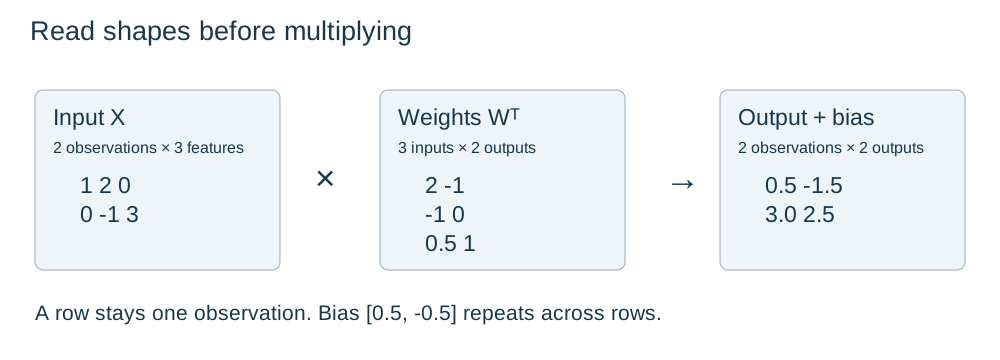
A neural network begins with ordinary numbers arranged according to a contract. The arrangement tells the program which numbers belong to one observation and which numbers are features of that observation. If that contract is wrong, a program can produce valid arithmetic for the wrong question. Reading shapes is therefore part of understanding a model, before any discussion of accuracy.

Give each axis a meaning

A tensor is a numerical container with a shape. A scalar, such as one loss value, has shape (). A vector with three entries has shape (3,). A matrix with two rows and three columns has shape (2, 3). The number of axes is sometimes called the tensor's rank; this use of rank is different from matrix rank in linear algebra.

For tabular input, we use shape (B, D): B is the number of observations in the current batch and D is the number of features per observation. A batch groups observations for one computation. It does not create a new feature. If there are 12 observations with three measurements each, the shape is (12, 3), even if the training dataset contains thousands of observations.

A tensor does not know that a column means temperature. Keep the feature order alongside the data. Reversing two equally sized columns preserves shape while changing the question asked of every learned weight. Numerical shape checks and semantic checks are both necessary.

Work through one linear map

Let X name this two-observation input:

X = [[ 1,  2, 0],
     [ 0, -1, 3]]

We want two output numbers per observation. Let W be the weights, with one row for each output, and b be its two biases:

W = [[ 2, -1, 0.5],
     [-1,  0, 1.0]]
b = [0.5, -0.5]

A weight multiplies an input feature; a bias adds a value independently of the input. For each observation, multiply corresponding input and weight entries, add the products, then add the output's bias. The first observation's first output is 1×2 + 2×(-1) + 0×0.5 + 0.5 = 0.5. Its second output is 1×(-1) + 2×0 + 0×1 - 0.5 = -1.5.

For the second observation, the first output is 0×2 + (-1)×(-1) + 3×0.5 + 0.5 = 3. The second is 0×(-1) + (-1)×0 + 3×1 - 0.5 = 2.5. The output is therefore [[0.5, -1.5], [3.0, 2.5]], with shape (2, 2).

The compact expression is Z = X @ W.T + b. Z names the output, @ is matrix multiplication, and .T exchanges the two axes of this matrix. Shapes tell the same story: (2, 3) @ (3, 2) produces (2, 2). PyTorch's Linear(3, 2) stores its weights in shape (2, 3), matching the two rows of weights above. Although called a linear layer, its optional bias makes the transformation affine.

Check the arithmetic in PyTorch

import torch

X = torch.tensor([[1, 2, 0], [0, -1, 3]], dtype=torch.float32)
W = torch.tensor([[2, -1, 0.5], [-1, 0, 1]], dtype=torch.float32)
b = torch.tensor([0.5, -0.5], dtype=torch.float32)
Z = X @ W.T + b
expected = torch.tensor([[0.5, -1.5], [3.0, 2.5]])
assert X.shape == (2, 3)
assert Z.shape == (2, 2)
assert torch.allclose(Z, expected)
print(Z)

dtype describes the numerical representation. float32 is our usual training type; float64 provides extra precision for the tiny numerical gradient check later. Whole-number input written without a dtype may become an integer tensor, which is unsuitable for ordinary floating-point layer computations. Class-index labels will deliberately use an integer dtype in Lesson 02. Do not turn every tensor into floating point indiscriminately.

The device says where the tensor lives. This course uses the CPU. Compatible shapes alone are insufficient when operands have incompatible dtypes or devices. Check those properties when reading an error, instead of trying arbitrary reshapes.

Broadcasting can hide a wrong comparison

Adding b, shape (2,), to Z, shape (2, 2), repeats the same two biases across observations. This is intentional broadcasting. Broadcasting aligns dimensions from the right; dimensions must match or one must have size one.

Now imagine predictions of shape (3, 1) and targets of shape (3,). Subtraction can produce shape (3, 3), comparing each prediction with several targets. The arithmetic succeeds, but observation pairing is lost. For one-output regression, keep both tensors in shape (B, 1) and assert equality before computing the loss.

Likewise, reshape rearranges the view of stored values; it does not establish what an axis means. A transpose exchanges axes. Confusing those operations can scramble observations while retaining a plausible element count. Write the intended axis meanings first, then choose the operation.

Practice

Complete these before opening the solutions.

• 01A · A new observation: use X = [[2, 0, -1]] with the worked weights and biases. Predict the shape and calculate both outputs by hand; then verify them with PyTorch.
• 01B · A broadcasting trap: create predictions [[1.0], [3.0], [5.0]] and targets [2.0, 4.0, 6.0]. Inspect the subtraction's shape. Repair the target shape and explain which comparisons now occur.
• 01C · Count the adjustable numbers: a layer maps four features to three outputs with a bias. State the input, weight, bias and output shapes for a batch of five, and count its learned scalar parameters.

Exit check

Without running code, explain why Linear(3, 2) accepts (7, 3) and returns (7, 2). Then make your own one-observation example and verify each output independently. Passing these checks demonstrates shape reasoning for this layer; it does not yet demonstrate that you can train a useful network.

Further reading: PyTorch 2.9 Linear, tensor construction, and broadcasting semantics.

02 · Follow a prediction into its loss

Outcome: trace a forward pass and choose a loss whose inputs match the prediction task. Prerequisite: Lesson 01.

A forward pass is the computation that transforms input into a prediction using the current parameters. Nothing is learned merely because a forward pass happened. Learning requires measuring an error, finding how parameters affect that error and changing them. This lesson establishes the first two parts without hiding their meanings behind a training loop.

A small network with visible arithmetic

Let x = 2 be one input, w = 0.5 its first weight, and b = 0.1 the first bias. The first weighted sum is z = w×x + b = 1.1. The letter z names the value before activation.

Apply the rectified linear unit, or ReLU: h = max(0, z). Here max chooses the larger argument, so h = 1.1. The letter h names the hidden activation. With an output weight v = -1 and output bias c = 0.2, the prediction is yhat = v×h + c = -0.9. We write yhat for a prediction and y for the observed target.

ReLU leaves positive values unchanged and replaces negative values with zero. That change allows a network to behave differently in different input regions. Without an intervening nonlinear operation, a sequence of affine layers can be combined into one affine transformation. Adding layers alone would then add parameters without creating the nonlinear function family we need.

No activation is placed after this regression output: a continuous prediction may need to be negative. Output design follows the task. An attractive-looking diagram with the same activation everywhere is insufficient justification.

Squared error measures distance in target units

Suppose the observed target is y = 0.5. The prediction error is yhat - y = -1.4. For hand differentiation, we use L = 0.5×(yhat - y)² = 0.98, where L names the loss and the superscript two means square. The factor 0.5 simplifies the derivative in Lesson 03.

PyTorch's default MSELoss uses the mean of squared errors without that factor. For this single observation it returns 1.96. For predictions [1, 4] and targets [2, 2], the squared errors are 1 and 4, so their mean is 2.5. The mean is over all output elements. If a sample has several predicted values, those elements also enter the average.

For one-output regression, our contract is floating-point predictions (B, 1) and floating-point targets (B, 1). B is batch size. Matching those shapes prevents the cross-observation broadcasting mistake from Lesson 01. Squaring penalizes a two-unit error four times as much as a one-unit error; large errors therefore have substantial influence.

Binary classification starts with one logit

For two classes, we can produce one unrestricted real number per observation, called a logit. Sigmoid converts a logit a into p = 1 / (1 + exp(-a)), where p is the modeled probability of class 1 and exp is the exponential function. A logit of zero gives probability 0.5.

BCEWithLogitsLoss receives the raw logits and includes the needed probability transformation in a numerically stable computation. Do not apply sigmoid first. Our binary contract uses logits (B, 1) and floating-point labels of the same shape, with values zero or one. The loss also supports targets between zero and one, but this course's binary fixtures use hard labels.

For a class-1 observation, binary cross-entropy is -log(p), where log means natural logarithm. Probability 0.5 gives about 0.6931; probability 0.75 gives about 0.2877. Greater confidence in the correct class lowers this loss. A confidently incorrect prediction receives a larger penalty. Accuracy cannot express that distinction because it only counts the selected labels.

Several exclusive classes need several logits

For one of C mutually exclusive classes, emit C logits per observation. C means the number of classes. Use CrossEntropyLoss with logits (B, C) and integer class indices (B,) of dtype torch.long. In our class-index setup, valid labels run from zero through C - 1. Do not apply softmax before this loss.

Softmax converts scores into probabilities by exponentiating each score and dividing by the sum of those exponentials. For logits [log(2), 0, 0], exponentials are [2, 1, 1], giving probabilities [0.5, 0.25, 0.25]. A target of class zero gives loss -log(0.5), about 0.6931. The correct-class probability determines the unweighted single-example loss.

These classes are exclusive. A photograph that may contain both a bicycle and a dog poses a different, multi-label question. Do not select a loss solely from the number of label names.

import torch
from torch import nn

reg_pred = torch.tensor([[1.0], [4.0]])
reg_y = torch.tensor([[2.0], [2.0]])
assert reg_pred.shape == reg_y.shape
print(nn.MSELoss()(reg_pred, reg_y).item())

binary_logits = torch.tensor([[0.0], [1.0]])
binary_y = torch.tensor([[1.0], [0.0]])
print(nn.BCEWithLogitsLoss()(binary_logits, binary_y).item())

class_logits = torch.tensor([[1.0, 0.0, -1.0], [0.0, 2.0, 0.0]])
class_y = torch.tensor([0, 1], dtype=torch.long)
print(nn.CrossEntropyLoss()(class_logits, class_y).item())

Practice

• 02A · Follow the inactive path: repeat the scalar forward pass with x = -2, leaving all parameters and the target unchanged. Calculate z, h, yhat, half-squared loss and default MSE.
• 02B · Write three contracts: specify output shape, target shape, target dtype and loss for a batch of six house-price predictions, six binary ring labels, and six three-class observations.
• 02C · Confidence changes loss: using logits [log(2), 0, 0], calculate the loss when the target is class two. Explain why the prediction is unchanged but the loss differs from the worked class-zero case.

Exit check

For each code example, identify exactly what one output entry means. Explain why the hand-worked loss and MSELoss differ by a factor of two, and why displaying a binary probability requires a sigmoid while both classification training losses receive raw logits.

Further reading: PyTorch 2.9 ReLU, MSELoss, BCEWithLogitsLoss, and CrossEntropyLoss.

03 · Trace responsibility backward

Outcome: derive every parameter gradient in a scalar network, check it numerically and interpret one update. Prerequisite: Lessons 01–02 and the idea of a slope.

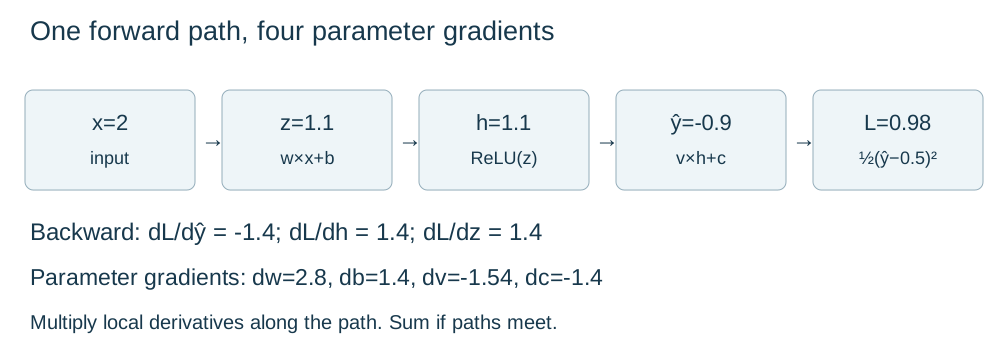
A loss says how far a prediction misses its target. It does not directly say which parameter to change. A derivative supplies local information: if one value changes by a small amount while other values stay fixed, how quickly does the loss change? Backpropagation organizes these derivatives through the computation that produced the prediction.

Keep the forward values on the page

Use the same network as Lesson 02: input x = 2, first weight w = 0.5, first bias b = 0.1, output weight v = -1, output bias c = 0.2, and target y = 0.5.

The forward steps are z = w×x + b = 1.1, h = max(0, z) = 1.1, and yhat = v×h + c = -0.9. The loss is L = 0.5×(yhat - y)² = 0.98. Here z is the pre-activation, h the hidden activation, yhat the prediction and L the loss. All four parameters are still at their original values.

We write dL/dw for the derivative of loss with respect to weight w, with the other parameters held fixed. In a multi-parameter setting these are partial derivatives; the collection of them is the gradient. A positive derivative means a sufficiently small increase in that parameter raises this loss locally.

Start at the error and follow each path

The derivative of half-squared error with respect to the prediction is the error itself: dL/dyhat = yhat - y = -1.4. Raising the prediction slightly would lower the loss, which matches the prediction being below the target.

The output is yhat = v×h + c. Increasing v changes the output at rate h = 1.1; increasing c changes it at rate one. The chain rule multiplies the rates along a path:

dL/dv = (dL/dyhat) × h = -1.4 × 1.1 = -1.54
dL/dc = (dL/dyhat) × 1 = -1.4
dL/dh = (dL/dyhat) × v = -1.4 × (-1) = 1.4

At z = 1.1, ReLU is on its positive branch, where changing z changes h at rate one. Therefore dL/dz = 1.4. Finally, the first weighted sum changes at rate x = 2 with respect to w, and at rate one with respect to b:

dL/dw = (dL/dz) × x = 1.4 × 2 = 2.8
dL/db = (dL/dz) × 1 = 1.4

The hidden derivative is positive even though the output derivative is negative. The negative output weight reverses the direction. Memorizing “the error gets sent backward” would miss this multiplication and produce the wrong first-layer update.

Check without trusting the derivation

A central finite difference estimates a derivative by evaluating the loss slightly above and below a parameter value. For weight w, the estimate is [L(w + eps) - L(w - eps)] / (2×eps). eps is a small positive perturbation; all other parameters remain unchanged. We use eps = 0.000001 and double precision to reduce rounding problems.

import math
import torch

values = [0.5, 0.1, -1.0, 0.2]  # w, b, v, c
params = [torch.tensor(t, dtype=torch.float64, requires_grad=True)
          for t in values]
w, b, v, c = params
prediction = v * torch.relu(w * 2.0 + b) + c
loss = 0.5 * (prediction - 0.5) ** 2
loss.backward()

def scalar_loss(p):
    w, b, v, c = p
    prediction = v * max(0.0, w * 2.0 + b) + c
    return 0.5 * (prediction - 0.5) ** 2

eps = 1e-6
expected = [2.8, 1.4, -1.54, -1.4]
for i, (name, parameter) in enumerate(zip(["w", "b", "v", "c"], params)):
    above, below = values.copy(), values.copy()
    above[i] += eps
    below[i] -= eps
    numerical = (scalar_loss(above) - scalar_loss(below)) / (2 * eps)
    automatic = parameter.grad.item()
    assert math.isclose(automatic, expected[i], abs_tol=1e-10)
    assert math.isclose(numerical, automatic, rel_tol=1e-6, abs_tol=1e-8)
    print(name, automatic, numerical)

Autograd records supported tensor operations and uses their derivatives during backward(). It differentiates the computation you wrote, including an incorrectly chosen loss. Numerical agreement is a local implementation check, not proof that the learning problem is well designed.

A perturbation that crosses ReLU's corner at zero can disagree with a single chosen derivative there. Extremely tiny perturbations also invite floating-point cancellation. Our example stays comfortably on the positive branch. Finite differences are useful for tiny checks but would require many forward evaluations for a large parameter set.

One simultaneous update

Plain gradient descent uses new parameter = old parameter - learning_rate×gradient. The learning rate controls the step size. At learning rate 0.1, the four new parameters are w = 0.22, b = -0.04, v = -0.846, and c = 0.34. Every update uses the gradients from the original forward pass; do not recompute only some gradients halfway through.

The new hidden value is max(0, 0.22×2 - 0.04) = 0.4. The new prediction is -0.846×0.4 + 0.34 = 0.0016, giving half-squared loss 0.12420128. Loss decreased on this observation. That alone says nothing about unseen data, and a much larger learning rate could overshoot.

Practice

• 03A · A different target: change only the target to y = -0.5. Derive the original-position loss and all four parameter gradients, then check them with finite differences.
• 03B · A closed gate: set w = -0.5, b = 0.1, keeping x = 2 and the original remaining values. Determine which gradients are zero and explain each zero through its path.
• 03C · Compare step sizes: from the original parameters, calculate one simultaneous update at learning rates 0.01, 0.1 and 1.0. Evaluate each new loss before interpreting which step helped most.

Exit check

Reproduce the four original gradients without code. Then run the numerical check and explain why changing the loss to default MSE doubles those gradients. If signs or factors disagree, identify the first local derivative where your calculation diverges.

Further reading: PyTorch 2.9 Tensor.backward and gradcheck.

04 · Decide what the model is allowed to learn from

Outcome: create fixed, disjoint splits, fit preprocessing on training observations and inspect batches without losing input–target pairing. Prerequisite: Lessons 01–03 and the train/validation/test distinction from Applied Machine Learning.

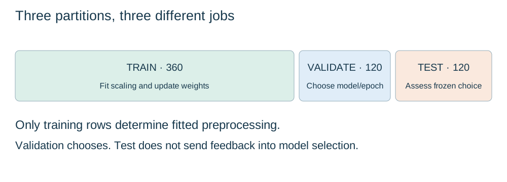
A correct derivative can optimize a misleading experiment. If information from the eventual test observations influences preprocessing or model choice, the reported score answers an easier question than prediction on genuinely unseen data. Data handling belongs inside the learning method, rather than being housekeeping before it.

Fix the evaluation question first

The core course fixtures contain independently generated synthetic observations. We assign 60% of their row IDs to training, 20% to validation and 20% to test, then preserve those memberships. An ID identifies an observation independently of its current position in a batch. Fixed membership lets us compare models against the same evidence instead of benefiting from a newly convenient split.

Training observations supply the optimization loss and preprocessing estimates. Validation observations guide choices such as learning rate, hidden width and stopping epoch. The test set is reserved for one final evaluation of the selected procedure. Repeatedly changing a model after reading its test result makes the test set part of development, even if no test gradient was computed.

Random row splitting fits the independent-sample setup here. It would not automatically fit repeated readings from the same patient, device or customer. If the intended prediction concerns unseen groups, keep groups separate. For prediction into the future, use a time-aware holdout. “Random” does not by itself mean “representative of the deployment question.”

Standardization is a learned transformation

Suppose a training feature has the two values 1 and 3. Its mean is 2. Its population variance is [(1-2)² + (3-2)²] / 2 = 1, so its population standard deviation is 1. Standardization subtracts that training mean and divides by that training standard deviation. The two transformed values are -1 and 1.

A later observation of 5 becomes (5-2)/1 = 3. We do not recompute a new mean using that observation. Otherwise the transformation would change with the evaluation batch, and a future observation would help determine how the model interprets itself.

For each feature, let mu name the training mean and scale its training population standard deviation. The transformed feature is (value - mu) / scale. The population convention divides squared deviations by the number of training observations. This is a scaling choice; we are not claiming to produce an unbiased estimate of an unknown population variance. In PyTorch, unbiased=False expresses this convention; the current documented spelling is correction=0.

If a feature is constant during training, its scale is zero. Dividing by zero creates invalid values. The example clamps scale to at least 1e-8, matching the staged checker and reference implementation, so constant training values become zero. A future departure from that constant can become very large after scaling; flag it for review rather than treating the clamp as a general solution. Record that condition: a constant training feature cannot teach the model how changes in that feature relate to the target.

Make the contract visible in code

This self-contained demonstration generates 100 independent synthetic sensor observations. The target combines a linear effect, a curved effect and fresh noise. The exact formula is for learning the workflow; it is not a physical model of a real sensor.

import torch
from torch.utils.data import TensorDataset, DataLoader

data_rng = torch.Generator().manual_seed(140)
X = torch.randn(100, 1, generator=data_rng)
y = 1.5 * X + 0.4 * X.square()
y = y + 0.1 * torch.randn(100, 1, generator=data_rng)

split_rng = torch.Generator().manual_seed(41)
ids = torch.randperm(100, generator=split_rng)
train_ids, val_ids, test_ids = ids[:60], ids[60:80], ids[80:]
assert len(set(ids.tolist())) == 100
assert not (set(train_ids.tolist()) & set(val_ids.tolist()))
assert not (set(train_ids.tolist()) & set(test_ids.tolist()))
assert not (set(val_ids.tolist()) & set(test_ids.tolist()))

mu = X[train_ids].mean(dim=0)
scale = X[train_ids].std(dim=0, unbiased=False)
scale = scale.clamp_min(1e-8)
train_X = (X[train_ids] - mu) / scale
val_X = (X[val_ids] - mu) / scale
train_data = TensorDataset(train_X, y[train_ids], train_ids)
val_data = TensorDataset(val_X, y[val_ids], val_ids)
train_loader = DataLoader(
    train_data, batch_size=16, shuffle=True, num_workers=0,
    generator=torch.Generator().manual_seed(42),
)
for batch_X, batch_y, batch_ids in train_loader:
    assert batch_X.shape == batch_y.shape
    assert batch_X.shape[0] == batch_ids.shape[0]
    print(batch_X.shape, batch_ids.tolist())

TensorDataset retrieves matching positions from its tensors. Keeping IDs in the example makes pairing inspectable. DataLoader groups retrieved samples into batches and shuffles training order when requested. It does not independently shuffle features and targets. With 60 training samples and batch size 16, the batch sizes are 16, 16, 16 and 12 when drop_last remains false.

An epoch is one traversal of the training loader. Shuffling changes order between epochs, not split membership. We leave validation and test order unshuffled and retain every observation. The CPU examples use num_workers=0 to keep loading easy to inspect. A seed helps reproduce a particular configuration; it does not guarantee identical results across every PyTorch release or device.

Practice

• 04A · Audit membership: write checks that the three split-ID sets are pairwise disjoint, have sizes 60/20/20, and together contain exactly IDs 0 through 99. Deliberately insert a duplicate across splits and confirm a check fails.
• 04B · Catch a leaking scaler: training values are [2, 4, 6] and one validation value is 20. Calculate train-only mean and population standard deviation, then transform 20. Compare with a scaler fitted to all four values and explain the information leak.
• 04C · Count batches: for 35 training observations and batch size eight, predict the batch sizes with drop_last=False and True. State which setting you would use for complete evaluation and why.

Exit check

Print one batch with its IDs and show that every target remains paired with its original observation. Then change validation feature values in a copy of the dataset and confirm that the already-fitted training mean and scale remain unchanged.

Further reading: PyTorch 2.9 data loading, standard deviation, and reproducibility; scikit-learn's data-leakage discussion.

05 · Give each training-loop line a job

Outcome: explain and implement a minibatch update, distinguish evaluation mode from disabled gradients, and aggregate loss correctly. Prerequisite: Lessons 01–04.

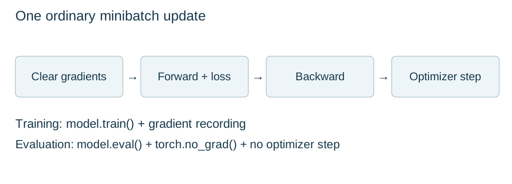
The training loop repeats the experiment from Lesson 03 on batches. Its brevity can make it tempting to memorize. Instead, follow what changes after each line. Predictions change when parameters change; gradients describe the current computation; and evaluation measures a fixed model without taking an optimization step.

From a gradient to an optimizer

An optimizer receives the parameters it is allowed to update. Plain stochastic gradient descent, or SGD, subtracts the learning rate times each current gradient. “Stochastic” reflects learning from sampled observations or minibatches rather than always using the complete dataset gradient. In our first examples there is no momentum or weight decay, so the update matches the arithmetic already derived.

Create the optimizer once after constructing the model. It must reference the model whose predictions enter the loss. Constructing a second model for the optimizer would leave the first model unchanged. Later optimizers may also retain useful state across steps, making unnecessary reconstruction another source of error.

Read one step in causal order

Start with model.train() to select training behavior. Then optimizer.zero_grad(set_to_none=True) clears gradients left from the previous update. Calculate predictions, calculate the scalar loss, call loss.backward() to obtain gradients, and call optimizer.step() to change parameters.

backward() accumulates into parameter gradients. Without clearing them, a second step can use a mixture of current and stale gradients. Accumulation can be deliberate in more advanced workflows; here it would violate the intended one-batch update. Clearing immediately before each forward pass is an easy convention to audit. Clearing after backward but before the optimizer step discards the gradients the step needs.

The forward pass builds a new computation graph for the current parameters and batch. Do not compute one loss outside the loop and repeatedly call backward on that old computation. Ordinary training does not need retain_graph=True.

A small, complete loop

This miniature linear dataset is an arithmetic diagnostic, separate from the course's held-out sensor experiment. Its four training points follow y = 2×x + 1. There is no claim here about performance on unseen observations.

import torch
from torch import nn
from torch.utils.data import TensorDataset, DataLoader

torch.manual_seed(7)
X = torch.tensor([[-1.0], [0.0], [1.0], [2.0]])
y = 2 * X + 1
loader = DataLoader(TensorDataset(X, y), batch_size=3, shuffle=True,
                    generator=torch.Generator().manual_seed(8))
model = nn.Linear(1, 1)
loss_fn = nn.MSELoss()
optimizer = torch.optim.SGD(model.parameters(), lr=0.05)

for epoch in range(100):
    model.train()
    loss_total, observation_count = 0.0, 0
    for batch_X, batch_y in loader:
        optimizer.zero_grad(set_to_none=True)
        prediction = model(batch_X)
        assert prediction.shape == batch_y.shape
        loss = loss_fn(prediction, batch_y)
        if not torch.isfinite(loss):
            raise RuntimeError("Non-finite training loss")
        loss.backward()
        optimizer.step()
        count = batch_X.shape[0]
        loss_total += loss.item() * count
        observation_count += count
    epoch_training_loss = loss_total / observation_count

model.eval()
with torch.no_grad():
    final_prediction = model(X)
    final_training_mse = loss_fn(final_prediction, y).item()
print("Final training MSE:", final_training_mse)
print("Weight and bias:", model.weight.item(), model.bias.item())

The loop uses default mean MSE with one predicted value per observation. Multiplying each batch mean by its observation count reconstructs its sum of squared errors. Summing those contributions and dividing by the total count gives the correct observed-sample average. If four observations have mean loss one and the final single observation has loss nine, the overall mean is (4×1 + 1×9)/5 = 2.6. Averaging the two batch means would incorrectly give five.

During training, different batches see slightly different parameter values because updates occur between them. The accumulated training loss therefore describes that traversal. Re-evaluating all training observations after the epoch describes the final fixed model, which need not produce the identical number.

Evaluation has two separate switches

model.eval() selects evaluation behavior in layers that distinguish it, including dropout and batch normalization. It does not turn off gradient recording. torch.no_grad() disables gradient recording for operations inside its context, reducing unnecessary tracking during evaluation. It does not select evaluation behavior. Use both when evaluating the course models.

For a network containing only linear layers and ReLU, train/eval mode may not change its predictions. Keeping the distinction explicit prepares you for layers where it matters. Before the next training epoch, call model.train() again. For validation, use the frozen training preprocessing and the validation loader; omit backward and optimizer steps. Test evaluation follows the same computational pattern only after model selection is finished.

Debug the first batch before waiting for epochs

Check prediction shape, target shape, finite values and loss definition first. Inspect a parameter before and after one step to establish that an update occurred. If loss becomes non-finite, investigate inputs, scaling and learning rate before trying a larger network. A simple model should usually be able to fit a tiny, suitable diagnostic dataset, but that test does not measure generalization.

A learning rate that is too large can bounce across useful parameter regions; one that is too small can make progress hard to see. Do not interpret every short-term rise in minibatch loss as failure. Compare epoch-level training and validation behavior while preserving the validation/test roles.

Practice

• 05A · Explain the broken order: consider loss.backward(); optimizer.zero_grad(set_to_none=True); optimizer.step(). Explain what information is discarded and write a correct order for one ordinary update.
• 05B · Weight the final batch: three batches contain four, four and two observations, with mean losses 0.5, 1.0 and 3.0. Compute the full-dataset mean and compare it with the unweighted mean of batch means.
• 05C · Verify a mode distinction: use a Linear(1, 1) model in evaluation mode on an input while gradient recording is enabled. Inspect the output's requires_grad. Repeat inside torch.no_grad() and explain the difference.

Exit check

Run the diagnostic, then explain why a small final training MSE alone is insufficient evidence for deployment. On a fresh single batch, show that gradients exist after backward and at least one parameter changes after the optimizer step.

Further reading: PyTorch 2.9 SGD, zero_grad, module modes, and no_grad.

06 · Ask what extra flexibility actually buys

Outcome: compare a linear baseline with a small nonlinear model using a fixed evaluation plan, and explain the geometry of a ring classifier. Prerequisite: Lessons 01–05 and baseline evaluation from Applied Machine Learning.

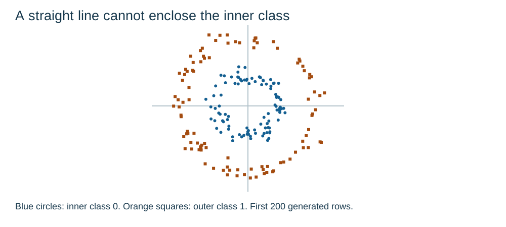
A deeper model is useful only when its additional flexibility addresses a relevant limitation and survives evaluation. Begin with a model simple enough to understand. It establishes a reference score and exposes data or training problems that additional layers could hide. This lesson joins two small questions: predicting a continuous sensor response and classifying concentric rings.

First establish the regression baseline

The sensor fixture relates two measured inputs to a continuous response, with a squared effect of the first input and independent noise. Fit an intercept-only reference using the training-target mean, then fit a linear regression model using Linear(2, 1) and MSELoss. Both use the same fixed split IDs. Standardize both features using training statistics; keep the target in its original units so the error remains interpretable.

The constant reference asks how much improvement comes from using the input at all. The linear model asks how much a straight trend captures. Calculate validation MSE for selection and, when reporting results, also consider mean absolute error, the average absolute prediction error. MSE squares target units; mean absolute error retains the target's units. Neither describes the cause of the relationship.

To see a linear limitation without training anything, take hypothetical inputs [-1, 0, 1] and targets [1, 0, 1]. A constant prediction of 2/3 gives squared errors 1/9, 4/9 and 1/9; mean error is 2/9. Symmetry makes the best least-squares line horizontal here. Increasing training time cannot make that line bend downward in the middle.

These three points are an arithmetic illustration, not a claimed score on the sensor fixture. On actual validation observations, inspect residuals as well as an average. Residual means observed target minus prediction. A curved residual pattern provides a specific reason to consider a nonlinear candidate. A larger model's lower training error alone does not.

Hidden units make several local rules possible

A multilayer perceptron, abbreviated MLP, combines affine layers with nonlinear activations. With one hidden layer, each hidden unit receives a weighted sum of the input and applies ReLU. The final layer combines the resulting activations.

For one input, ReLU creates a change of slope where its weighted input crosses zero. Several hidden units can place changes at different positions, approximating a curve over the observed range. In two dimensions, these become changes across regions. Extrapolation still needs separate justification.

import torch
from torch import nn

linear_regressor = nn.Linear(2, 1)
linear_classifier = nn.Linear(2, 1)
ring_classifier = nn.Sequential(
    nn.Linear(2, 16), nn.ReLU(),
    nn.Linear(16, 16), nn.ReLU(), nn.Linear(16, 1),
)

assert linear_regressor(torch.zeros(4, 2)).shape == (4, 1)
assert linear_classifier(torch.zeros(4, 2)).shape == (4, 1)
assert ring_classifier(torch.zeros(4, 2)).shape == (4, 1)
assert sum(p.numel() for p in ring_classifier.parameters()) == 337

Sequential passes each layer's output into the next. This course comparison uses two hidden layers: 48 parameters in the first layer, 272 in the second and 17 in the output, totaling 337. The linear classifier has three. The regression MLP uses the same dimensions but a different loss. Extra parameters create flexibility and additional estimation demands.

Why rings are a useful challenge

Each ring observation has two coordinate features. One class lies near an inner circle and the other near an outer circle, with independently generated variation. A one-logit linear classifier predicts from a×x1 + b×x2 + c. Here x1 and x2 are the two coordinates, a and b are their weights, and c is a bias.

At the default probability threshold 0.5, a zero logit marks the boundary. The equation a×x1 + b×x2 + c = 0 describes a straight line when the feature weights are not both zero. A straight line cannot surround the inner ring while excluding the outer ring everywhere. Training longer cannot remove that representational limitation.

ReLU hidden units combine several regions, allowing a small MLP to approximate an enclosing boundary. Train it with BCEWithLogitsLoss using floating-point binary labels shaped (B, 1). For a default label prediction, compare its logit with zero; apply sigmoid only when you need a displayed probability. Keep any threshold choice part of validation-based selection, not test-based adjustment.

Compare procedures, not lucky runs

Keep split IDs, preprocessing rules, metric definitions and the candidate budget fixed. Record the model, initialization seed, learning rate, batch size and stopping rule. Use validation results to choose between candidates and restore the selected parameter state before the final test. If early stopping is used, the final training epoch may not contain the selected model.

The supplied comparison selects by validation loss. Also compare accuracy with a majority-class reference chosen from training labels. Inspect a confusion matrix: true/predicted class counts can expose neglect of one class. These synthetic results do not certify real-world performance.

Use a small, declared candidate set. Repeated validation selection can overfit the development evidence. Test once after fixing the procedure and report the result without silently replacing inconvenient outcomes.

Practice

• 06A · Count a smaller candidate: count the parameters in Linear(2, 1) and in a 2–16–1 MLP with ReLU. Compare the latter with the displayed 2–16–16–1 model. Explain which additional capability depends on ReLU.
• 06B · Explain the boundary: sketch ideal circles of radii one and two. Draw a straight decision boundary, identify where it must fail, and describe why a collection of piecewise-linear regions could help.
• 06C · Make a selection plan: specify a comparison of the linear and MLP ring classifiers, including fixed data, training-only preprocessing, one primary validation metric, a stopping rule and the point at which the test set may be evaluated. Do not invent performance numbers.

Exit check

Explain a plausible observation that would justify trying the MLP and one that would make you investigate the pipeline first. For each candidate, state its exact output/loss contract and identify the evidence needed before claiming an improvement.

Further reading: PyTorch 2.9 Sequential and Linear; scikit-learn's common evaluation pitfalls.

07 · When fitting better means predicting worse

A model can become increasingly accurate at reproducing its training rows while becoming less useful on new rows. This is not a contradiction. Training asks an optimizer to reduce one finite collection of errors. Generalization asks whether the resulting rule survives another sample from the intended population. Those are related goals, not identical goals.

Suppose a sensor reading contains a stable pattern plus measurement noise. With enough flexibility, a network can fit both. A future measurement contains different noise, so copying the training noise is wasted effort. We call this overfitting. The evidence is not merely “the network has many parameters.” Look for a meaningful training–validation gap under comparable measurement conditions, and for validation performance worsening as training continues. A gap can also arise from distribution shift, different label quality or a bug. Diagnose before prescribing.

Compare comparable curves

Our training loop records two training losses. The online training loss is accumulated while parameters are changing and dropout may be active. The evaluation-mode training loss is measured after the epoch with one fixed parameter state and dropout disabled. Validation is measured the same way. Compare evaluation-mode training loss with validation loss when diagnosing fit. A lower validation loss than online training loss is not automatically leakage: the online calculation may have been deliberately harder.

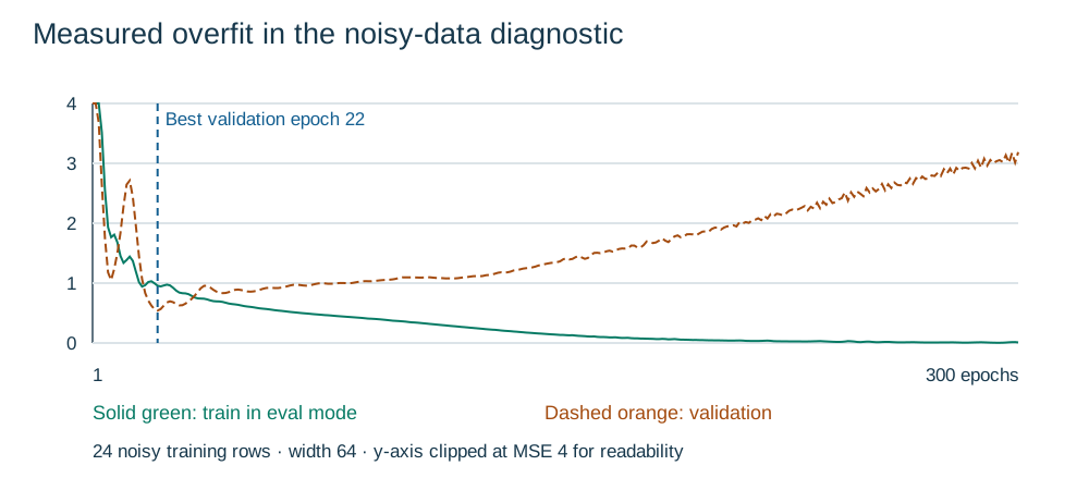
The chart is generated from actual course runs. Its horizontal axis is epoch, meaning a complete pass through the training rows. Its vertical axis is mean loss. The highlighted epoch is the lowest observed validation loss within the declared training budget. The curve after that epoch still matters: it shows why keeping the final weights can be a different decision from keeping the best validation checkpoint.

Run python -m dlcourse.diagnostics. The small-noisy-training case deliberately keeps only 24 training rows and adds noise to their targets. Validation retains the original process. Compare the wider network with a narrower regularized candidate. This is a diagnostic stress test, not a claim about all regression problems. The script honestly reports whether regularization wins here; do not rewrite the story to guarantee a preferred result.

Three different interventions

A smaller model restricts the set of functions that can be fitted. It may reduce overfitting, but it can also underfit a real nonlinear relationship. A linear model that cannot separate concentric rings needs a better representation, not merely more epochs.

Weight decay shrinks parameters during optimization. In AdamW, the decay is separate from the adaptive gradient calculation. With learning rate 0.01 and decay coefficient 0.1, the decay-only multiplier for a weight is 1 - 0.01*0.1 = 0.999 for that step. A weight of 2 becomes 1.998 before considering the gradient contribution. This is a small cumulative pressure, not a rule forcing all weights to zero. It is not interchangeable with every implementation of adding an L2 penalty to an adaptive optimizer. Our teaching model applies decay to all parameters for simplicity; advanced practice often uses parameter groups.

Dropout randomly suppresses intermediate values during training. With probability 0.25, a value is zeroed; retained values are multiplied by 1/0.75. For an input value 3, the training output is either 0 or 4. Its expectation is still 3. At evaluation, ordinary dropout is the identity operation. This is why model.eval() is part of the inference contract. Dropout is not a guarantee of better results and need not help a tiny clean dataset.

Checkpoint selection limits how long a fitted trajectory is allowed to keep adapting to training details. Our implementation trains the full budget and restores the best validation checkpoint; it does not stop computation early. A patience-based early-stopping loop would save computation, but the selection criterion must still be fixed without consulting test results.

Validation is a resource

Trying fifty combinations and selecting the best noisy validation score can itself overfit validation. The core course declares just two candidates per task and a fixed epoch budget. Report what was tried, including the losing baseline. For serious studies, use the cross-validation and nested-evaluation ideas from Applied ML, or reserve additional evaluation data appropriate to the deployment question. Do not “repair” a disappointing test score by choosing another checkpoint using that test score.

Exercises

• 7A · Dropout expectation. With dropout probability 0.4 and input value 6, list the possible training outputs and their probabilities. Compute their expected value and the evaluation output.
• 7B · Choose a checkpoint. Validation losses at epochs 10, 20, 30, 40 are 0.48, 0.31, 0.35, 0.39. Training losses keep falling. Which checkpoint does the declared minimum-loss rule choose? Why is “epoch 40 has lowest training loss” insufficient?
• 7C · A controlled experiment. Read the noisy-case configuration and final history rows. Write a four-sentence comparison naming sample size, candidate differences, best validation epoch and the limitation created by changing several regularization choices together.

Exit check: explain why no_grad() does not disable dropout, and distinguish best-checkpoint restoration from actual early stopping.

08 · Debug the learning process before enlarging the model

A falling loss is reassuring only after you know what loss was actually computed. A shape bug can optimize the wrong comparison; leakage can make a weak model look excellent; a disconnected graph can leave parameters unchanged. Practical deep learning starts with small checks that separate these causes. A larger network usually makes a broken experiment harder to understand.

Begin with a contract

Print one batch's feature shape, target shape, dtype and finite-value range. For the rings classifier, features are [batch, 2], logits and floating targets are [batch, 1], and targets contain only 0 or 1. For bars, features are [batch, 1, 8, 8], logits are [batch, 2] and integer class indices are [batch]. The same word “classification” does not imply interchangeable shapes.

Now check the first prediction and loss. At binary logit zero, sigmoid is 0.5 and binary cross-entropy is approximately 0.693147 for either class. At two equal class logits, categorical cross-entropy is also approximately 0.693147. This gives a useful scale for an initially uncertain classifier. It is not a required initial value: random weights may produce unequal logits.

The diagnostic script deliberately subtracts predictions [3,1] from targets [3]. The result is a [3,3] matrix of all pairwise differences. Predictions 1, 2, 3 perfectly match their own targets, yet the wrong broadcasted MSE is 4/3 instead of zero. Broadcasting is useful when intended, but a valid tensor operation is not proof of valid statistics. Shape assertions are cheap insurance.

Follow one update

Record a parameter before the training step and after optimizer.step(). If it never changes, inspect whether it belongs to the optimizer, whether the loss depends on it, whether gradients exist, and whether training accidentally runs inside no_grad(). A parameter can legitimately have zero gradient in one batch, especially behind an inactive ReLU, so inspect a few meaningful examples rather than declaring a global bug from one zero.

Next inspect gradient clearing. For L = w² at w = 1, one backward pass adds gradient 2. A second backward pass on a newly computed loss, without clearing gradients, adds another 2, giving 4. This is accumulation, not a recalculation that replaces the old gradient. Accumulation can be deliberate for micro-batches, but then the scaling and update schedule need an explicit design. Our simple loop clears gradients before every batch.

Make the problem intentionally easy

Try fitting a handful of clean training examples. If a sufficiently flexible model cannot reduce their loss, investigate implementation before generalization. Check that labels correspond to the correct rows, the loss matches the task, the output activation is correct, and the optimizer sees the parameters. Passing this test only establishes learning mechanics. It says nothing about held-out performance.

The five-point examples/03_miniloop.py is such a mechanics test. Its target is exactly 2*x + 1. Its fitted weight should be close to 2 and bias close to 1. We deliberately avoid calling its training fit a test result.

Recognize unstable updates

For the toy objective L = 0.5*w², the derivative is w. One SGD step gives w_new = (1 - learning_rate)*w. A learning rate of 0.5 halves the magnitude every step. A learning rate of 2.2 changes its sign and multiplies its magnitude by 1.2, so the squared loss grows by 1.44 each step. Run the large-step diagnostic and verify that pattern. This exact threshold belongs to this particular quadratic; do not apply “learning rate below 2 is safe” to arbitrary neural networks.

When a real loss becomes non-finite, inspect inputs, target scaling, loss usage and learning rate. Shrinking the learning rate may help, but can also hide a shape or preprocessing error. Gradient clipping limits update-driving gradient magnitudes in some settings; it is not included in the core implementation because the first task is to identify the cause.

Metrics tell different stories

The rings report includes true negatives, false positives, false negatives and true positives. At the fixed probability threshold 0.5, predicted class 1 means logit at least zero. Precision asks what fraction of predicted positives are correct; recall asks what fraction of actual positives are found. The report uses zero when a denominator is zero and documents that convention. Accuracy alone can conceal a model that predicts only a majority class. These synthetic classes are approximately balanced within random splits, but that is not an assumption for real work.

Inspect errors against input location or image orientation on validation first. Do not use the test set as an interactive debugging dashboard. A surprisingly perfect synthetic result can simply mean the toy task is easy. It does not demonstrate safety, fairness, calibration, real image recognition or readiness for deployment.

Exercises

• 8A · Broadcast trap. Write the 3-by-3 difference matrix for predictions and targets 1, 2, 3. Calculate its MSE and explain why a diagonal-only comparison is intended.
• 8B · Update or no update? Name three distinct causes of unchanged parameters and a concrete observation that distinguishes each.
• 8C · Confusion counts. For TN=60, FP=10, FN=20, TP=30, calculate accuracy, precision and recall. What changes if the cost of false negatives rises?

Exit check: present a debugging order that starts with data/shape checks and reaches model capacity only after the basic update is verified.

09 · A tiny convolutional network you can account for

Flattening an image makes it usable by an ordinary linear layer, but it discards explicit neighborhood structure. Pixel 17 and pixel 18 may be adjacent; pixel 17 and pixel 49 may not be. A convolutional layer applies a small learned pattern detector repeatedly across local neighborhoods. Reusing the same weights across positions is the key structural assumption. A horizontal edge should be recognizable in more than one part of an image.

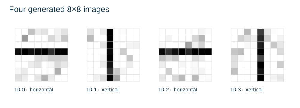
We use 8-by-8 grayscale images generated entirely in the course. Each image contains a noisy horizontal or vertical bright bar. Class 0 is horizontal; class 1 is vertical. Positions vary, noise is independent and pixel values are clipped to known bounds 0–1. This dataset is intentionally small enough to inspect, generate and train on CPU. It does not stand in for medical images, handwriting or real camera scenes.

Compute one local response

Consider the 3-by-3 image patch with rows [0,0,0], [1,1,1], [0,0,0]. A horizontal-line kernel with the same three rows produces response 3: multiply corresponding entries and add them. A vertical-line kernel with rows [0,1,0], [0,1,0], [0,1,0] produces response 1 on that patch. A bias, if present, is added after the sum. The numbers illustrate a possible detector; actual training learns its own weights and need not reproduce these exact kernels.

PyTorch calls the layer Conv2d, though its numeric operation is cross-correlation: it does not flip the kernel as a strict mathematical convolution definition would. This distinction matters when checking arithmetic by hand, but the learned-weight idea is the same.

A channel is one feature plane. Grayscale input has one channel. Four learned kernels produce four output channels, each potentially responsive to a different pattern. More channels are not more training examples. The batch axis still counts examples.

Account for every dimension

The model uses Conv2d(1,4,kernel_size=3,padding=1), ReLU, MaxPool2d(2), flattening and a linear head. For batch size 5:

• Input: [5,1,8,8]
• Convolution: [5,4,8,8]
• ReLU: [5,4,8,8]
• Two-by-two max pooling with stride 2: [5,4,4,4]
• Flatten from dimension 1: [5,64]
• Linear layer to two class logits: [5,2]

With dilation 1, output width is floor((input_width + 2*padding - kernel_width)/stride) + 1. Here it is (8+2-3)/1+1 = 8. Without padding, it would be 6. Max pooling keeps the greatest value in each non-overlapping two-by-two neighborhood. That reduces resolution; it can preserve a strong local response while losing its exact position. Pooling does not guarantee invariance to every shift, and boundaries still matter.

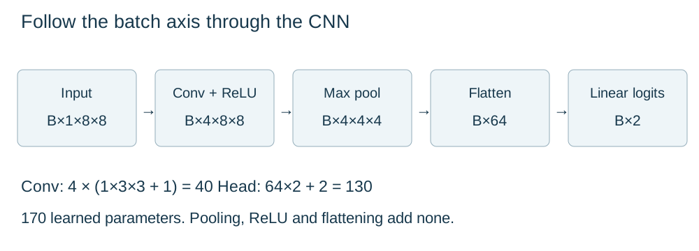
Count parameters rather than guessing from layer count. Each convolutional output channel has 1*3*3 = 9 weights and one bias. Four channels give 40 parameters. The linear head has 64*2 = 128 weights and two biases, giving 130. Total: 170. ReLU, max pooling and flattening have no learned parameters. python -m examples.04_cnn_shapes checks both dimensions and count.

Train with the same experimental discipline

The targets are integer class indices, so the head returns raw logits and the loss is CrossEntropyLoss. Do not add a final softmax before that loss. Softmax is useful when presenting relative class probabilities after training. Argmax of logits already gives the same most-probable class without an extra softmax calculation.

Run python -m dlcourse.run --task bars. The declared candidates are a flattened linear classifier and the tiny CNN. Each uses only training rows for updates, validation loss selects its checkpoint, and the winning candidate is selected before the test calculation. The flattened baseline matters: if a simple model works as well, a CNN may not be necessary for this task. More complicated architecture is not an automatic achievement.

Inspect false positives and false negatives on validation. Ask whether errors depend on bar position or noise, and whether a proposed augmentation preserves labels. Horizontal or vertical translation can preserve orientation. A 90-degree rotation swaps horizontal and vertical, so retaining the old label would corrupt this particular task. Augmentation is a statement about the meaning of the target, not a universal checklist.

Exercises

• 9A · Local detector. Compute the horizontal and vertical kernel responses on a vertical center-column patch. Assume zero bias.
• 9B · Shape change. Remove convolution padding but keep the rest of the architecture. Find the new feature shape after pooling and the required input dimension of the final linear layer.
• 9C · Label-preserving transforms. Classify horizontal flip, 90-degree rotation and mild added sensor noise as safe, label-changing or assumption-dependent for this dataset. Explain each decision.

Exit check: derive the 170-parameter count without running code, and state why success on these generated bars does not validate real-world computer vision.

10 · Turn a successful run into a reproducible experiment

A notebook that once printed a good score is a weak scientific record. To understand what happened later, you need the data-generating process, row assignments, preprocessing state, model definition, optimization settings, selection rule and measured result. Reproducibility makes the experiment inspectable; it does not make the underlying prediction problem valid automatically.

Our package records seed 2718 for generated data and 2719 for the split permutation. Each task contains 600 examples: 360 train, 120 validation and 120 test. The training seed and loader shuffle seed are also explicit. Data rows are given stable IDs before shuffling, so a split can be checked for overlap rather than trusted by description. data/manifest.json records shapes and CSV checksums. The reference program generates the same float32 data directly; CSV files are human-inspectable exports using enough significant digits for float32 round trips.

Randomness has several homes

A data generator, parameter initializer and minibatch shuffle each consume random numbers. If all three share one implicit stream, an innocent extra random draw can change the rest of the experiment. Dedicated generators make these dependencies clearer. The course uses an explicit generator for data, another for split IDs and another for each training loader. Global framework randomness is still seeded for model initialization and dropout.

A seed is not a promise that every machine, library release or hardware backend produces identical results. The verified path is CPU, one thread, Python 3.12 and PyTorch 2.9.1+cpu. Deterministic algorithms are requested. Different operating systems or library builds may change floating-point details; meaningful comparisons should use stated tolerances, not insist every decimal match. Keep environment version records and separate numerical regression checks from statistical claims.

Save the right state

A PyTorch model architecture describes operations. Its state dictionary contains learned tensors and registered buffers. To resume optimization exactly, optimizer state also matters: AdamW remembers running gradient statistics. An epoch counter and random-number generator states can matter too. The core course saves reports and retrains small models quickly rather than distributing binary checkpoints. This keeps the learner package source-only and avoids teaching untrusted model loading casually.

When keeping a best checkpoint in memory, a shallow reference to the current state can accidentally keep changing during later training. Our loop makes a deep copy when validation improves, then reloads it at the end. That is why the final reported validation loss matches the minimum saved history value even when the last epoch is worse.

If you later save and load weights, use trusted files and follow the current official serialization guidance, including restricted loading where appropriate. Do not download and execute arbitrary model artifacts simply because they have a familiar extension. The course requires no pretrained downloads.

Separate reproducibility from test reuse

The reference scripts may be rerun to verify the same frozen teaching experiment. This is not new evidence from fresh test data. The test partition remains the same 120 examples, and repeated executions do not increase its sample size. If you inspect the reference test score and then use it to redesign your own model, that partition is no longer a clean final assessment of your redesign.

For the capstone, document your protocol before running final evaluation. Keep a modest predeclared candidate set, select with validation and state any earlier exposure to the bundled test result. An instructor can generate a fresh hidden assessment set from a new seed after the model choice is frozen. It must have the same intended data process, and its labels must not become tuning feedback. This is a pedagogical assessment practice, not a substitute for a realistic deployment dataset.

Write a result someone can challenge

An honest report names the task, baseline, split, selected model, selection rule, result and limitations. “The network learned rings” is less useful than “On this fixed balanced class-conditional synthetic rings experiment, the validation-selected MLP achieved the reported accuracy on 120 held-out samples using a threshold fixed at 0.5.” State the actual measured value from your report, not one copied from a lesson. Give confusion counts alongside a rounded percentage so the reader can see the denominator.

The uncertainty of a result is not captured by a deterministic seed. The synthetic sample is only one sample, the generator is only one world, and no real deployment distribution has been established. Real applications also need privacy, fairness, monitoring, security, maintenance, cost and human oversight decisions. Those topics are important precisely because a good local metric does not settle them.

Exercises

• 10A · Missing record. A teammate saves only a model state dictionary and a test score. Name five missing pieces required to understand or reproduce the experiment.
• 10B · Best weights. Explain why storing best_state = model.state_dict() without a deep copy can be dangerous during continued training. Identify the relevant line in our implementation.
• 10C · Same test twice. You rerun the frozen reference experiment and obtain the same accuracy. Does the effective test sample become 240? Explain what this rerun actually verifies.

Exit check: distinguish run reproducibility, fresh-sample uncertainty and generalization to a new real-world population.

11 · Two bridges beyond the core: reuse and attention

This lesson gives concrete mental models for two common extensions. It does not train a production vision system or a language model. You already know enough to ask better questions about them: what representation is computed, which parameters are updated, how data is split and what is actually evaluated?

Transfer learning reuses a representation

Imagine a network separated into a feature extractor and a prediction head. The extractor maps an input to a feature vector; the head maps that vector to the target required by the current task. In transfer learning, some parameters were learned on a source task before adaptation to a target task. A useful source representation can reduce target-data requirements, but success depends on how relevant the source and target are. “Pretrained” does not mean universally suitable.

The simplest adaptation freezes the extractor and trains a new head. Setting the extractor parameters' requires_grad to false prevents their gradients being recorded for optimization. Constructing the optimizer from only trainable parameters makes the intended update scope explicit. That still leaves a separate question about module mode. An extractor containing dropout or batch normalization can behave differently in training mode even when its weights are frozen. For a fixed feature extractor, keep it in evaluation mode while training the head. Calling model.train() on the entire parent module can accidentally switch it back.

Fine-tuning instead allows some source parameters to change. This increases flexibility and can erase useful representations if adaptation is too aggressive. Learning rates, layer selection and checkpoint choice belong to validation decisions. The original source training data may overlap an evaluation dataset, so provenance matters as well as code.

The runnable examples/06_freeze_features.py uses a small, explicitly handcrafted extractor. It verifies which parameters change and demonstrates the mode boundary. It is a mechanics demonstration, not an empirical transfer-learning result, because those extractor weights were not learned on a source dataset. We deliberately make that distinction rather than download a large model and imply the difficult evaluation problem has disappeared.

Sequence data introduces order and variable length

A sequence is an ordered collection, such as readings over time or token IDs in a sentence. A typical hidden-state tensor is [batch, sequence_length, features]. Padding can make different lengths fit one rectangular batch, but padding positions should not become meaningful evidence. A mask tells an operation which positions to ignore. For prediction over time, the split must also respect the direction of information: a feature from tomorrow cannot help a model that must decide today.

Attention builds a weighted combination of value vectors. A query expresses what the current position is looking for; keys are compared with that query; the resulting scores become nonnegative weights summing to one; values are averaged using those weights. These names describe different roles, not separate databases or hidden intelligence.

Consider query [1,0], two keys [1,0] and [0,1], and values [2,0] and [0,4]. Dot products are 1 and 0. With key dimension 2, scaled scores are 1/sqrt(2) and 0, approximately 0.7071 and 0. Softmax exponentiates and normalizes them, producing weights approximately 0.6698 and 0.3302. The result is approximately [1.3395,1.3210]. It is a blend of the two values, with more weight on the key that matched the query better.

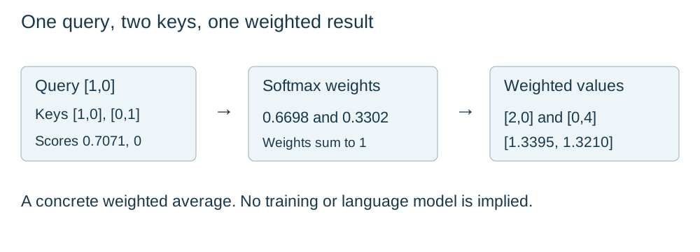
Run python examples/05_attention_arithmetic.py and compare the numbers. In a learned model, linear projections usually produce queries, keys and values from representations. In a causal next-token model, positions must not attend to future tokens; an attention mask removes that information path before normalization. An unmasked demonstration of two keys is not an implementation of a causal language model.

Know what is still missing

A transformer combines attention with additional operations, including position information, feed-forward transformations, residual connections and normalization. Multiple heads allow several learned comparison spaces. Training a useful language model also requires tokenization, a suitable objective, substantial data, compute, evaluation and safety work. Reading one weighted-average example does not establish transformer implementation competence, much less LLM mastery.

Attention weights can help inspect a computation, but they are not automatically a faithful explanation of a prediction or proof of causal importance. A model's behavior depends on all its transformations. Carry forward the same habits from this course: inspect shapes, track information availability and make claims only at the scale of the evidence.

Exercises

• 11A · Freeze is not eval. A frozen feature extractor contains dropout. Why can repeated outputs still differ? What two separate settings should you inspect?
• 11B · Equal attention. If both scores are zero and values remain [2,0] and [0,4], compute weights and output. Explain why the output is not either original value.
• 11C · Future leakage. A model predicting the next token allows the current position to attend to later ground-truth tokens during training. Explain why this changes the prediction problem and how a causal mask addresses the information path.

Exit check: state exactly what the frozen-extractor and attention scripts demonstrate, and one major capability neither establishes.

12 · Defend one small neural experiment end to end

The capstone is a compact research report, not a race for the largest model. Your job is to make one prediction task understandable, reproducible and honestly evaluated. A modest score with a sound protocol is more valuable than a spectacular score obtained by tuning on the test set. You will build on the supplied components, but you must make and explain the important choices yourself.

Choose the regression task as the default path. Its two inputs are fictional standardized sensor-like measurements and its target is a continuous response. The generating process contains a linear contribution, a quadratic contribution and random noise. Because this is synthetic, you can compare the model's behavior with the known construction without pretending to have discovered a physical law. The optional extension is the rings classifier. Complete one coherent experiment before adding another.

Stage 1: make a contract before a model

Write a question in plain language: what does one row represent, what inputs are available, what target is predicted and what kind of new examples should performance describe? Record the IID assumption. Explain that a random row split would be inappropriate if several rows came from one person/device or if deployment predicts future periods with changing conditions. In those situations, return to the group/temporal evaluation material from Applied ML.

Declare split seeds, counts and selection metric. For regression, validation MSE is the selection criterion; RMSE and MAE help communicate performance in target units. Fix a small candidate set before using final test results. Include the train-mean baseline and a linear neural layer. Your nonlinear candidate must be small enough to train on CPU. Record every candidate you actually try.

Stage 2: implement and inspect

Complete the five public stages in exercises/stages.py. Run python check_learner.py; its default imports your functions, not the reference functions. Passing these checks is necessary but not sufficient. The checker verifies shape, preprocessing, model output and update mechanics. It cannot judge whether your written deployment question is sensible.

Next edit exercises/capstone.py, supplying your planned candidate configurations and report rationale. Run python -m exercises.capstone to produce training/validation evidence only. It should record row IDs, training-only scaling, candidate histories and the chosen index. Read those results and write your choice down. Do not run final evaluation simply because training finished if the protocol is still changing.

A common temptation is to fix the input scale using all 600 rows because “there are no labels in the mean.” That still lets the held-out feature distribution influence the fitted pipeline. Fit the scaler only on training rows. Reuse its mean and scale on validation, test and future inputs. The same principle applies to learned imputations and feature selection, not just normalization.

Stage 3: freeze, then assess

Finalize the candidate list and selected model using validation. Save the exact plan and its hash. Then run the explicit --final mode once to evaluate the selected configuration on the test partition and write the final report. The course runner includes guardrails against accidentally overwriting final results. These guardrails are not cryptographic secrecy: the bundled data and reference outcomes are visible. Disclose any prior test exposure rather than pretending the learner package provides a hidden benchmark.

A final score cannot tell you whether the architecture was well chosen for every plausible future task. Compare it with the naive baseline and your declared expectations, show the sample count, and explain whether the result supports the narrow question you asked. If test performance disappoints, report it. Further redesign requires a new evaluation plan and fresh held-out data, not quietly recycling this test set as validation.

Stage 4: explain an error and a limitation

Choose a diagnostic using validation data: inspect residuals across the first input, compare easy/hard regions of the rings, or inspect image errors by bar position in the optional extension. Identify one plausible cause and one experiment that could distinguish it from an alternative. Avoid claiming a causal explanation solely from a pattern in errors.

Your final report should be short enough for a reviewer to understand without reading every source file. Include a model shape trace, one correctly worked gradient example, learning curves, the selection rule, final metrics and a limitations paragraph. Link the exact configuration and generated outputs. State the actual environment tested. “Works on my CPU” is a useful verified statement; “works everywhere” requires evidence you do not yet have.

Exercises

• 12A · Protocol audit. A learner compares four candidates on test accuracy and reports only the best. Rewrite the procedure to preserve a final assessment boundary.
• 12B · Evidence package. List the files a reviewer needs to reproduce your training/validation selection and understand the final result. Distinguish them from a virtual environment or downloaded wheel, which should not be submitted.
• 12C · Responsible conclusion. Write a two-sentence conclusion that includes task, split, baseline comparison and one limitation. Use your actual measured results, not a promised improvement.

Exit check: another learner can reproduce your selection from the source and explain why no test result drove that selection. Use CAPSTONE.md for the full deliverable contract and rubric.

Synthetic data and provenance

All three datasets are original generated teaching fixtures. There are no real people, customers, medical records or operational measurements. dlcourse/core.py::generate is the authoritative generator; python -m tools.export_data reproduces the CSVs and manifest. Training generates these tensors directly rather than reading mutable CSV files.

Each task has 600 row IDs and a deterministic random 60/20/20 train/validation/test split. IDs are local to a task. The same split permutation across tasks does not link the fictional observations semantically. Regression rows are IID. Classification features are independent conditional on fixed alternating class labels, with 300 examples of each class before random splitting. Grouped or time-dependent data needs a different design.

• regression.csv: row_id, split, x0, x1, target. Inputs are uniform on [-2,2]; target is 1.5x0 - 0.7x1 + 0.9*x0² plus Gaussian noise with standard deviation 0.15. All units are fictional arbitrary units.
• rings.csv: row_id, split, x0, x1, target. Alternating labels generate 300 examples of each class before splitting; random angle and noisy radii around 0.7 and 1.5 give concentric rings. Labels are 0 inner, 1 outer. Radius noise standard deviation is 0.12.
• bars.csv: row_id, split, x0…x63, target. Flattened 8×8 grayscale arrays; row-major order reconstructs [1,8,8]. Random bar row/column is an integer 1…6; noise standard deviation 0.15 precedes clipping to [0,1]. Labels are 0 horizontal, 1 vertical.

CSV uses nine significant digits for float32 export. Feature standardization for regression/rings uses only the 360 training rows. Bars use known clipping bounds rather than a fitted scaler. Test rows remain visible for reproducibility; this is a teaching fixture, not a secure hidden examination. manifest.json contains hashes and feature/target shapes.

Validation and remaining gaps

Executed evidence · 2026-10-14

• Python 3.12.14, Linux x86_64, actual PyTorch 2.9.1+cpu; CPU only, one thread, deterministic algorithms requested
• Isolated validation environment, with system-site-packages disabled; exact versions recorded in outputs/environment-packages.json; pip check passed
• 14 reference unit tests passed, covering split disjointness/completeness, generator repeatability, train-only scaling, constant features, shape contracts, exact backprop, loss values, eval/no-grad behavior, confusion counts, checkpoint reproducibility, sample-weighted aggregation and stage reference
• All six example programs and six lesson Python blocks executed successfully
• All three full training tasks executed; an independent review reran them twice and reproduced every candidate history, selected epoch and test value exactly in this environment
• Five staged learner functions checked separately; the incomplete starter fails intentionally. Ten deliberately broken/starter variants were rejected after strengthening the public checker
• Independent CSV audit matched all exported float32 features/targets, hashes and split IDs to generated tensors
• Independent capstone probes confirmed selection is unchanged when test tensors are replaced with NaNs, final evaluation requires matching selection, and a second final invocation refuses overwrite
• All diagnostic cases executed, including the honest case where regularization did not beat the best checkpoint of the wider model
• 161 static source/HTML/asset checks passed; independent review confirmed all local targets/fragments, heading structure, prompt/answer counts and chart points
• All nine SVG diagrams were rendered with Inkscape and visually inspected for clipping, spacing and mathematical labels. Browser rendering remains unverified.

This evidence is from actual PyTorch execution. NumPy is an installed interoperability dependency; no NumPy implementation is substituted for the framework.

Measured outputs and tolerances

Reference full three-task internal runtime was about 4.95 seconds in the first run, excluding interpreter startup. Independent reruns took about 5.2–5.3 seconds internally and 6.8–7.0 seconds including startup. These are authoring-machine measurements, not timing promises for learner devices.

Regression selected MLP: test RMSE 0.161159, MAE 0.125866; train-mean baseline test RMSE 2.285362. Rings selected MLP: 120/120 correct. Bars selected CNN: 120/120 correct. Test labels contain 57 class-zero and 63 class-one samples. The bars linear candidate also had perfect validation accuracy; CNN selection reflects lower validation loss. Perfect toy scores support no claim of real-world perfection.

Within the exact same verified environment, reruns matched exactly. For supported but different CPU builds, use absolute tolerance 1e-5 for deterministic small numerical checks where documented, and diagnose rather than blindly fail if full-training metrics change slightly. A practical reference comparison band is ±0.02 RMSE or ±0.02 accuracy, not a statistical confidence interval or universal pass requirement. Different versions or architectures can alter optimization enough to need a new reference record. Hand backprop/finite-difference checks use float64 and tighter explicit tolerances.

Installation footprint and scope

The official CPU torch wheel was 184,378,187 bytes. Initial dependency downloads totaled approximately 211 MB from rounded installation logs; the later ignore-installed resolution check downloaded approximately another 211 MB to validate package availability. No GPU or torchvision packages were installed. Final environment logical size was 905,253,518 bytes (about 863 MiB), excluding external interpreter targets. Exact footprint is recorded in outputs/runtime-footprint.json. Runtime binaries, wheels, virtual environments, checkpoints and caches are excluded from the learner archive.

The distributed CPU requirements were resolved with pip from the official PyTorch/PyPI indexes. The isolated environment was assembled in two installation steps, then checked against these requirements; a second newly created environment was not installed solely to repeat identical downloads. macOS requirements and Windows commands were reviewed but not executed. The chosen historical stable version is pinned for reproducibility, not claimed newest.

Explicit unverified areas

No user Mac, VPS or live site was modified. No publication occurred. Real Windows/macOS installation, mobile-browser interaction, full browser navigation/printing, screen-reader behavior, hosted-notebook execution, integration with the existing Aabha lab, and a beginner learner pilot remain unverified. An attempted headless Chromium launch failed because the cloud sandbox disallowed its socket creation; no browser rendering pass is claimed. Static link/markup checks and local image inspection are not accessibility certification. Suggested pacing and grading thresholds have not been piloted.

Before release, verify the actual supported learner platforms, keyboard/screen-reader access, mobile reflow, download paths and lab runtime. Keep the numerical and evaluation-integrity tests when editing content or upgrading dependencies.

Source register and attribution

Checked 2026-10-14. Text, exercises, code, diagrams and data are original teaching work; external documentation is linked rather than copied. Examples are not adapted from proprietary course material. Documentation supports API contracts; measured outputs come from this package's executed programs. Timings and grading standards are author proposals, not external research findings.

Version policy: the verified baseline is PyTorch 2.9.1+cpu and Python 3.12.14. Versioned 2.9 API pages avoid confusing a moving latest-docs build with the tested runtime. The official previous-versions page lists this stable release and CPU installation route. No claim that 2.9.1 is the latest release is made.

Primary references by teaching purpose

• Installation and exact stable CPU release: PyTorch previous versions
• Tensor constructor/dtypes: torch.tensor, Lesson 01
• Stored linear weight dimensions: nn.Linear, Lessons 01/06
• Broadcasting semantics: broadcasting notes, Lessons 01/08
• Rectified activation: nn.ReLU, Lessons 02/03
• Regression reduction: MSELoss, Lesson 02
• Binary raw-logit contract: BCEWithLogitsLoss, Lesson 02
• Multiclass indices/raw logits: CrossEntropyLoss, Lessons 02/09
• Reverse-mode derivative API: Tensor.backward, Lesson 03
• Finite-difference checking guidance: gradcheck, Lesson 03
• Dataset and loader contracts: data loading, Lesson 04
• Standard-deviation correction: torch.std, Lesson 04
• Leakage and train-only fitting: scikit-learn common pitfalls, Lessons 04/06/12
• Basic optimization step: SGD, Lessons 03/05/08
• Gradient clearing: Optimizer.zero_grad, Lessons 05/08
• Mode/state/parameter APIs: nn.Module, Lessons 05/10/11
• Suppressing autograd recording: no_grad, Lesson 05
• Composing modules: Sequential, Lesson 06
• Decoupled weight decay implementation: AdamW, Lesson 07
• Dropout training/evaluation behavior: Dropout, Lesson 07
• Cross-correlation and image shapes: Conv2d, Lesson 09
• Determinism boundaries and seeds: reproducibility notes, Lesson 10
• Feature extractor versus fine-tuning framing: official transfer-learning tutorial, Lesson 11. The course does not execute its downloaded-model path.
• Original transformer architecture reference: Vaswani et al., Attention Is All You Need, Lesson 11. Our two-key arithmetic illustrates one attention operation, not the paper's full trained system.

Original artifacts and limits

The scalar chain-rule example, synthetic generators, all nine SVG visuals, diagnostic cases, assessment prompts and capstone are original. No external images, model weights or datasets are redistributed. Diagrams have descriptive text and SVG title/description fields, but assistive-technology behavior has not been certified. The independent review and validation record separate actual execution evidence from proposed classroom/platform behavior.

Instructor guide

The learner is expected to know Python arrays/functions and basic supervised evaluation. Use the readiness diagnostic before Lesson 01. If shape reasoning is weak, work on paper before adding training. If chain-rule arithmetic is weak, keep the four-parameter network visible and multiply one path at a time. Calculus notation is introduced locally; no proof-heavy prerequisite is assumed.

Suggested sessions pair reading, hand calculation, prediction-before-run and a small code change. Ask learners to explain why an output should change before they run the program. Do not grade copied reference scores as implementation understanding. Use the public checker for stage mechanics and the rubric for experimental judgment.

Key misconceptions to surface: tensor rank versus matrix rank; nn.Linear stores transposed weights relative to X@W notation; [B] and [B,1] can broadcast incorrectly; half-squared loss differs from MSE; classification losses consume raw logits; zero_grad after backward discards needed gradients; eval is not no_grad; freezing is not eval; last epoch is not always the selected checkpoint; repeated test runs are not more test observations; synthetic perfection is not production validation.

The regularization stress test is intentionally nuanced: the wider network overfits badly by the last epoch, but its best validation checkpoint can still beat the regularized candidate. Teach the observed result instead of promising that dropout/decay always improve performance. Several hyperparameters differ between these two stress candidates, so the result does not isolate the causal effect of one intervention.

Core reference code is readable source. It uses only CPU and local generated data. Before classroom use, verify installation on the actual learner machines, keyboard/browser navigation, diagram readability, screen-reader alternatives and the time required for learners to complete stages. These checks and a beginner pilot have not been performed. Suggested pacing and scoring cutoffs are author choices, not validated learning-outcome measurements.

Assessment privacy: use fresh instructor-held data only if you have a suitable delivery process. The course fixture is public to its recipients and does not provide secrecy. Never describe the code guardrails as preventing a determined learner from accessing test labels. They prevent common accidental workflow mistakes.

Publication readiness requires editorial review, actual website integration, mobile/browser and accessibility QA, installation trials and a learner pilot. This package has not been published. Any live lab integration must explicitly provide PyTorch or clearly label the practice as external/local; a generic browser Python editor is insufficient evidence.