
SQL · Module 11
Prepare AI features without future leakage
Estimated study time: 75–105 minutes. Read, predict, run, explain, then attempt the independent work.
SQL often supplies a machine-learning dataset. Before choosing a model, decide what one training row represents and when the prediction would have been made. Here the illustrative question is: among customers already registered before 1 March 2025, who will place a completed order during March? One row represents an eligible customer at the 1 March cutoff.
A feature is information available at that prediction time. A label is the future outcome we later observe. We will use January and February completed-order counts, sales before refunds and recency as features. The label is whether the customer buys during March. The code that constructs those two pieces must keep their time boundaries separate.
The feature query starts with eligible_orders, selecting only completed orders dated before 1 March and no earlier than 1 January. It aggregates lines to order grain, then orders to customer grain. A final left join begins from the eligible customer population, retaining customers who have no qualifying orders. Eren is registered before the cutoff but has only a pending February order, so the feature row has zero completed orders and zero sales.
Recency is the days from the last qualifying order to the cutoff. Eren has no such order, so recency is null. Replacing it with zero would incorrectly mean “ordered on the cutoff day.” A downstream model may need an imputation rule and a missingness indicator, but that is a separate modeling decision learned on training data. The SQL extraction should preserve the meaning first.
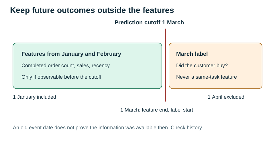
Read the diagram explanation
Feature window is January 1 inclusive to March 1 exclusive. Prediction is at March 1. Label window is March 1 inclusive to April 1 exclusive. Use only information available at prediction time.
A date filter alone cannot recover history
The fixture assumes that a stored completed status was known on the order date and that relevant records arrived without delay. That is a simplifying teaching assumption. A real database often stores current status only. If an order was pending on 28 February but completed on 3 March, using today's completed status can leak future information even when order_date is before 1 March. A genuine historical feature table needs status-effective times or trustworthy as-of snapshots, plus source availability timestamps when late arrival matters.
The same concern applies to refunds, customer attributes and corrected records. Our chosen sales feature deliberately uses line sales before refunds and is named accordingly. It is not the quarter's net-sales metric from the capstone. A production net-spend feature would need refunds observable before the prediction cutoff, not all refunds known today.
Keep population and outcome definitions aligned
The label query uses the same eligible customers as the features, then searches only March completed orders. Customers who registered on or after 1 March are excluded from both sides. Gita, registered exactly on 1 March, is not silently added because she exists in today's customer table. Join features to labels on customer_id and verify that both sides have exactly one row for each eligible key.
Do not feed bought_in_march, March order counts or March revenue back into the feature columns. Those describe the outcome you are trying to predict. Also avoid using identifiers as unexplained predictive signals, including unnecessary names, or exporting personal details simply because they are available. This exercise needs customer_id only for alignment; it is not automatically a useful model input.
The six-row fixture teaches extraction mechanics. It is far too small to establish model quality, fairness or a business-ready recommendation. A real project needs an appropriate population, time-based evaluation, leakage checks and a documented data-access basis. SQL correctness is necessary for that work, but it does not make the learning problem valid by itself.
Worked example 11 features
Follow the two aggregation stages and then the population-preserving join. The expected six rows include Eren with null recency. Farah’s February 28 order is one day before the cutoff.
WITH eligible_orders AS (
 SELECT o.order_id,o.customer_id,o.order_date,
 SUM(i.quantity*i.unit_price-i.line_discount) AS sales_before_refunds
 FROM aabha_sql.orders AS o JOIN aabha_sql.order_items AS i ON i.order_id=o.order_id
 WHERE o.status='completed' AND o.order_date >= DATE '2025-01-01'
   AND o.order_date < DATE '2025-03-01'
 GROUP BY o.order_id,o.customer_id,o.order_date
), customer_features AS (
 SELECT customer_id,COUNT(*) AS completed_orders,
 SUM(sales_before_refunds) AS sales_before_refunds,MAX(order_date) AS last_order_date
 FROM eligible_orders GROUP BY customer_id
)
SELECT c.customer_id,COALESCE(f.completed_orders,0) AS completed_orders,
 COALESCE(f.sales_before_refunds,0) AS sales_before_refunds,
 DATE '2025-03-01'-f.last_order_date AS recency_days
FROM aabha_sql.customers AS c LEFT JOIN customer_features AS f ON f.customer_id=c.customer_id
WHERE c.signup_date < DATE '2025-03-01'
ORDER BY c.customer_id;
Expected result from the bundled dataset:
| customer_id | completed_orders | sales_before_refunds | recency_days |
|---|---|---|---|
| 1 | 1 | 320.00 | 55 |
| 2 | 2 | 1640.00 | 15 |
| 3 | 1 | 520.00 | 29 |
| 4 | 1 | 450.00 | 28 |
| 5 | 0 | 0 | NULL |
| 6 | 1 | 360.00 | 1 |
The runnable file is sql/examples/11_features.sql.
Worked example 11 labels
The March outcome is separate. It must never be used as an input feature for the same March prediction.
SELECT c.customer_id,
 CASE WHEN EXISTS (SELECT 1 FROM aabha_sql.orders AS o WHERE o.customer_id=c.customer_id
 AND o.status='completed' AND o.order_date>=DATE '2025-03-01'
 AND o.order_date<DATE '2025-04-01') THEN 1 ELSE 0 END AS bought_in_march
FROM aabha_sql.customers AS c WHERE c.signup_date<DATE '2025-03-01' ORDER BY c.customer_id;
Expected result from the bundled dataset:
| customer_id | bought_in_march |
|---|---|
| 1 | 1 |
| 2 | 1 |
| 3 | 1 |
| 4 | 1 |
| 5 | 1 |
| 6 | 0 |
The runnable file is sql/examples/11_labels.sql.
Independent practice
11a
Count customers eligible for a prediction at 1 March using the stated registration rule. Name the result eligible_customers.
Hint: A customer registered exactly on the cutoff is outside the before-cutoff population.
11b
Wrap the supplied feature query in a features CTE and compare its row count with COUNT(DISTINCT customer_id). Return rows and distinct_customers. Then write one paragraph naming two real-world leakage risks this static fixture cannot resolve.
Hint: Remove the inner query’s final semicolon before enclosing it in a CTE. Matching counts check uniqueness, not time validity.
Check before moving on
You can identify the prediction time, feature window, label window, population and observation-history assumption. Do not claim a production-ready training dataset from this fixture.
Read the separate answers and explanations
Reading progress
13 lessons remain open to guests. Marking a lesson read records reading only; it does not award assessment credit or a certificate.
Device reading marks require browser storage. Reading is always available.
Sign in or create an account to save separate account progress. Your current page is kept.
Your earlier place on this device suggests these lessons. No new lesson is marked read.