Explained practice and checkpoint answers
Attempt the learner workbook first. Answers explain the method and the limits of the claim, not merely the numerical result. Reasonable alternative wording and chart choices are acceptable when the question, units and assumptions stay correct. The capstone reference follows these answers; it is a comparison model, not text to submit as your own.
Lesson 1 answers
1A. The 340-row count answers “How many joined tracking-event rows are present?” assuming each joined row is one event. The fraction of shipments late requires one late status per shipment and a denominator of 100 evaluable shipments. Repeated events from one shipment neither create new shipments nor provide independent copies of the outcome.
1B. Three of six evaluable shipments are late: 50%. “Three of six shipments with known timing were late; two of eight had unknown timing.” If both unknowns are on time, the all-eight rate is 3/8=37.5%; if both are late, it is 5/8=62.5%. These are possible-value bounds, not a sampling interval.
1C. One defensible contract: describe recorded reliability among 240 shipments in fictional weeks 1–8, unit=shipment, outcome=actual_minutes > promised_minutes, comparing standard with priority. Report group counts and route mix. Service choice is observational, so the difference does not isolate a causal service effect. Actual time alone ignores different promises.
Lesson 2 answers
2A. Sum=110, mean=110/6=18.333… minutes. Median remains (10+11)/2=10.5. Linear Q1=9.25, Q3=11.75 and IQR=2.5 remain unchanged because their interpolation uses middle values. The tail change raises the mean and range but not these rank-based summaries. This robustness does not justify ignoring the 60 minutes when estimating total workload.
2B. A fence identifies unusually positioned observations, not proven errors. Deleting all flagged values changes the population being described and can hide genuine long jobs. Preserve raw data, investigate flagged cases, correct only with evidence, retain plausible values in the primary result and label any sensitivity analysis. “True average” overstates what exclusion establishes.
2C. A is concentrated at 3; B is polarized between 1 and 5. A category-count plot or individual dots on the ordered 1–5 scale makes this visible. The shared mean does not establish similar satisfaction distributions; the scale's ordinal nature also calls for care with equal-spacing interpretations.
Lesson 3 answers
3A. Duration distribution: equal-bin histogram, x=minutes, y=shipment count. Late by service: category bars or dots, y=late percentage and labels=count/denominator. Over weeks: line chart, x=ordered week and y=late percentage, with denominators. Distance versus duration: scatterplot, x=km and y=minutes. Other well-labelled designs can work if they preserve the intended comparison.
3B. Use a zero-baseline bar chart with values 48% and 52%, and supply the actual group counts/denominators rather than inventing them. A defensible title is “Recorded rate differs by 4 percentage points”; the outcome and period must be added when known. The rates did not double: 52/48≈1.083, an 8.33% relative increase. The truncated baseline inflated the visual ratio.
3C. “In this separate illustrative table, East had 18/120 late shipments (15%) and West had 12/120 (10%), so West’s observed rate was 5 percentage points lower. Route and service mix may differ, so this descriptive comparison does not establish a causal hub effect.” This communicates the important comparison without depending on color.
Lesson 4 answers
4A. Random assignment supports an intervention comparison among enrolled units under assumptions such as adherence, no interference and comparable outcome measurement. Volunteer recruitment from one shift limits population coverage. Differential dropout, spillover between groups or changing the measurement method for one group could compromise the comparison.
4B. Respondent mean=32/8=4.0. Lowest all-ten mean=(32+2×1)/10=3.4; highest=(32+2×5)/10=4.2. These bounds enumerate possible missing values on the allowed scale; they do not express 95% repeated-sampling coverage or indicate which values are likely.
4C. Outcomes from the same person may share ability, habits or conditions. Four people provide four person-level units, with repeated observations that may be correlated. Ask how assignment occurred, how tasks are ordered, whether conditions changed, and what dependence structure is plausible. A repeated-measures or clustered design needs suitable methods; treating 40 rows as independent can understate uncertainty.
Lesson 5 answers
5A. Delayed: 160 flagged, 40 unflagged. Non-delayed: 80 flagged, 720 unflagged. Total flagged=240, so 160/240=66.67% of flags identify delayed jobs. Sensitivity and false-positive rate match the lesson, but the larger base rate raises the positive predictive fraction.
5B. Probability no delivery is late is 0.9³=0.729. At least one late is 1−0.729=0.271, or 27.1%. Multiplication assumes the three outcomes are independent and the per-delivery probabilities are 0.10 under this toy model. Shared conditions could invalidate it.
5C. P(late given priority)=4/20=20%; P(priority given late)=4/28≈14.29%; P(priority and late)=4/100=4%. The first denominator is priority shipments, the second late shipments, and the third all shipments. Reversing a condition changes the question.
Lesson 6 answers
6A. SE=6/√9=2 minutes; at n=36, SE=6/6=1 minute. The individual SD is still assumed to be 6. The estimate's repeated-sample variability shrinks because more independent outcomes are averaged, not because individual outcomes become less variable.
6B. Three of nine means equal 4, giving 1/3. Means at least 5 occur in (4,6), (6,4), (6,6), giving 3/9=1/3. The population mean is fixed at 4 in the specified finite population. These probabilities concern random samples and their means, not uncertainty about that known population mean.
6C. Repeats may share the same underlying participant value or measurement condition. Independence has not been established, and duplicate or correlated measurements do not supply the information of new independent participants. Repeats can improve some measurement estimates, but a suitable design/model must account for within-unit dependence.
Lesson 7 answers
7A. SE=4/√16=1 minute. Margin=2.131×1=2.131 minutes. Interval=[17.869,22.131] minutes, about [17.87,22.13]. State that this is an interval for the model population mean under independent normal observations with unknown variance, not for individual durations.
7B. Correct wording: “This 95% confidence-interval procedure covers the fixed mean in about 95% of repeated samples under its assumptions.” It does not assign a frequentist 95% probability to the fixed mean after observing this particular interval. It also does not describe the fraction of individuals within the bounds; that would involve the outcome distribution or a prediction/tolerance method.
7C. The 99% interval is wider because the procedure needs a larger allowance to achieve higher long-run coverage. Precision and coverage trade off for the same data. Neither interval automatically corrects selection bias, missingness bias, model misspecification or measurement error.
Lesson 8 answers
8A. “The checklist group averaged 3.2015 minutes less than control, a checklist−control difference of −3.2015. The 95% Welch interval was [−5.8496,−0.5534] minutes and the two-sided p-value was 0.0191 under the equal-mean null model. The calculation assumes independent outcomes from the specified model, and the entirely simulated study provides no direct evidence of real operational effectiveness.” Rounded equivalents are appropriate in a management brief.
8B. No. The interval permits a 6-minute reduction and a 4-minute increase. Non-rejection of zero does not establish equality, absence of a useful effect or equivalence. An equivalence claim needs a justified pre-specified acceptable range and a method designed for that claim.
8C. Different independent people in two assigned groups can fit Welch's setup if outcome assumptions are suitable. Before/after data from the same people are paired and need a method respecting those pairs. Team-randomized tasks are clustered at the assignment unit; an independent-task Welch analysis ignores team dependence. Changing the numerical method does not fix a flawed recruitment or measurement process.
Lesson 9 answers
9A. Absolute change=9%−12%=−3 percentage points. Relative change=(9−12)/12=−0.25=−25%. “Down 3%” could mean 3 percentage points or 3% of the baseline, which would be a much smaller change. Write the units and the baseline.
9B. At 80% short and 20% long, A=0.8×90%+0.2×10%=74%; B=0.8×95%+0.2×20%=80%. The equal-mixture rates were 50% and 57.5%. Both targets favor B, but the absolute rates and differences change because the target route mix changes. Standardization is a descriptive comparison for the specified mixture; it does not automatically identify a causal hub effect.
9C. The interval excludes zero and lies on the lower-duration side. It does not establish a reduction of at least 2 minutes because it includes −0.55, which corresponds to a smaller benefit. A real controlled pilot with a stated practical threshold, cost/quality measures and an appropriate design is more defensible than claiming a full rollout is proven worthwhile by simulated data.
Lesson 10 answers
10A. Fitted value=12.6622+1.8058×40=84.8942 minutes, approximately 84.89. Residual=90−84.8942=+5.1058 minutes. The hypothetical shipment was about 5.11 minutes slower than the line's fitted value. Using full-precision coefficients gives a slightly different last decimal, which is rounding rather than a method disagreement.
10B. Correlation does not establish cause. r is not a percentage of delay explained, and the fitted outcome is actual delivery minutes, not the late indicator. The dataset is fictional and observational. A better sentence: “Recorded distance and actual minutes have a strong positive linear association in this synthetic fixture, r≈0.923; route/service mix and shared weekly conditions limit causal and inferential interpretation.” R²≈0.851 describes in-sample variation around the mean, not a causal share.
10C. Zero and 100 km lie outside the observed range, so intercept interpretation and a 100-km prediction require extrapolation assumptions. Look for curvature, changing residual spread, unusual influential observations and patterns by time or service. A high R² does not rule them out.
Lesson 11 answers
11A. Example: “Investigate route and service mix before ranking the hubs. In the 240 recorded synthetic shipments from weeks 1–8, East averaged 79.63 minutes and West 45.96, but East's routes averaged 36.85 km versus 18.67 km and priority shares differed. Late rates were much closer: 25/120 at East and 26/120 at West. These descriptive results do not isolate a causal hub effect. Compare similar service and route groups, review promise definitions and check whether those groups have adequate overlap. Ratings also need a coverage warning because 41 of 240 are missing, with more missingness among late shipments. The current file can guide questions for investigation, but cannot establish that changing hub management will improve outcomes.”
11B. The first is an observation. The second is an interpretation based on selective nonresponse plus the relationship between late status and observed ratings. The third is a recommendation. The missingness pattern suggests a risk; it does not reveal the exact missing ratings or prove the size of any bias.
11C. A causal hub ranking needs comparable design or justified adjustment beyond raw differences; “productivity” requires a defined output/input measure and the trial is simulated; a respondent average cannot automatically represent missing respondents. Repair: “West's recorded mean duration was lower, alongside shorter routes and a different service mix. The simulated checklist mean was about 13.35% lower than control, with uncertain practical benefit and no demonstrated real-world effect. The respondent mean rating was about 4.14 among 199 responses; 41 ratings were missing.”
Lesson 12 answers
12A. A good plan names the 240-shipment descriptive window, shipment grain, strict late boundary, independent simulated trial, checklist−control duration contrast and a 2-minute worthwhile threshold. It labels one additional shipment question exploratory. Preserve the initial plan, changes, reasons, dates and their effect on analysis scope. No single exact exploratory question is required.
12B. For “21.25% late”: source=data/shipments_clean.csv; unit=shipment; late=actual_minutes>promised_minutes; accepted timing records=240; late numerator=51; 51/240×100=21.25%; no additional exclusion. The raw audit reconciles to that clean file. A peer should reproduce both counts before rounding the percentage.
12C. The arithmetic mean of the 40 observed task values can remain a correct descriptive mean of tasks. An independent-person standard error, t-test and confidence interval would no longer have their stated design support because observations cluster within four people. Request the assignment unit and repeated-measure structure and use an appropriate design/method rather than relabelling rows as people.
Checkpoint marking guide
Award credit for sound reasoning in the learner's own words. Do not require verbatim wording. Each question's components sum to its stated points.
Checkpoint A answers 20 points
A1. One row per order versus one per joined item (1); denominator 80 evaluable orders (1); pre-aggregate/deduplicate by order while preserving outcome definitions (1).
A2. Mean=30/5=6 (1), median=4 (1), high 16 pulls mean upward while median depends on rank (1).
A3. Possible data-entry error (1), genuine long/difficult job or different process (1), investigate and document while retaining plausible unverified values in the primary result (1).
A4. Response fraction alone does not establish similarity between respondents and nonrespondents (2). Compare known characteristics or response rates by late status/service/other relevant measured categories (1), while acknowledging unobserved opinions remain unknown (1).
A5. Random sampling selects units from a target population (1) and supports population coverage/generalization under the design (1). Random assignment allocates intervention among enrolled units (1) and supports causal contrast under experimental assumptions (1).
A6. Histogram or appropriate individual-value plot (1); x=duration minutes, y=count for equal-bin histogram (1); a valid concern such as bin width, hidden tail, unequal-bin area or misleading scale (1).
Checkpoint B answers 20 points
B1. Total flags=135 (1), positive predictive fraction=40/135≈29.63% (1), 40/50=80% is the catch rate among delayed jobs (1).
B2. SE=8/√64=1 (1); SD describes individual variation (1); SE estimates repeated-sample variability of the mean under independence/model assumptions (1).
B3. Margin=2×2.1=4.2 (1); interval [25.8,34.2] (1); concerns the model mean, not individual durations (1); 95% describes procedure coverage under assumptions (1).
B4. Under the null model and assumptions, a statistic at least as extreme in either direction has probability 0.03 (2). Not probability the null is true (1), nor probability the effect is practically important or that a specific causal explanation is correct (1).
B5. Interval includes meaningful differences in both directions (1), non-rejection is not proof of equality (1), equivalence needs a pre-specified acceptable margin and suitable procedure (1).
B6. Selective reporting/multiple searching raises false-positive risk (1), disclose all analyses and label exploration (1), pre-specify a primary outcome or use suitable multiplicity control/independent confirmation (1).
Checkpoint C answers 20 points
C1. −2 percentage points (1); relative −20% (1); baseline explicitly 10% (1).
C2. Overall rates are weighted subgroup averages (1); group weights can differ by hub (1); an easy-route-heavy hub can rank higher overall despite lower rates within strata (1).
C3. One more km corresponds to 1.8 higher fitted minutes within the descriptive model (2). Does not show that shortening a route causally saves exactly 1.8 minutes (1).
C4. Any two, explained: curvature, heteroskedasticity/changing spread, dependence, omitted variables, influential points, poor out-of-sample performance (up to 3 for two sound explanations).
C5. Interval excludes zero (1), crosses −2 so worthwhile reduction not established (1), simulated evidence cannot prove real benefit (1), propose appropriately designed real pilot/measurement rather than guaranteed rollout (1).
C6. Names checklist−control and negative=faster (1), gives estimate and 95% Welch interval for mean difference (1), n=20 per group/40 total (1), labels simulated data and avoids individual/real-world guarantees (1).
Reference capstone for comparison after your attempt
There is more than one defensible recommendation. This example illustrates the evidence standard. Reproduce the values and critique the wording rather than copying it into your submission.
Plan and calculation record
Population for description: the 240 fictional recorded shipments in weeks 1–8. Unit: shipment. Late: actual_minutes strictly exceeds promised_minutes. Rating missingness does not invalidate otherwise valid shipment timing. Exploratory question: whether late shipments have different rating response coverage. Population for inference: repeated independent tasks under the simulated trial model, with 20 independent participants per randomized arm. Contrast: checklist minus control mean duration; negative means faster. Practical threshold: −2 minutes or lower, supplied for the exercise.
Raw accounting: 248 records = 240 accepted + 3 exact duplicates + 5 invalid extras. Six formatting cells were normalized and two stale late flags recomputed; these are cell-level corrections, not extra excluded rows. There are 240 distinct clean shipment IDs and 30 shipments per week. The raw file remains unchanged.
| Quantity | Reference result |
|---|---|
| Overall late | 51/240 = 21.25% |
| Actual duration | Mean 62.7942; median 62.2; sample SD 26.2236 minutes |
| Linear quartiles and IQR | Q1 45.05; Q3 77.975; IQR 32.925 minutes |
| East late / West late | 25/120=20.83% / 26/120=21.67% |
| East / West mean actual minutes | 79.6275 / 45.9608 |
| East / West mean distance km | 36.85 / 18.6725 |
| East / West priority share | 40/120=33.33% / 80/120=66.67% |
| Rating coverage | 199 responses, 41 missing out of 240 |
| Missing among late / on time | 20/51=39.22% / 21/189=11.11% |
| Respondent rating mean | 4.1357, on an ordered 1–5 scale |
| Trial control | n20, mean23.9895, sample SD4.1254 minutes |
| Trial checklist | n20, mean20.7880, sample SD4.1477 minutes |
| Checklist minus control | −3.2015 minutes; −13.3454% relative to control mean |
| Welch inference | SE1.3081; t−2.4475; df37.9989; two-sided p0.01912 |
| 95% difference interval | [−5.8496,−0.5534] minutes |
Appropriate charts: the supplied effect-interval design with a learner-authored caption; a two-category dot or bar display of missing-rating percentages by late status, labelled 20/51 and 21/189. For comparison after your attempt, assets/missingness.svg illustrates the second chart. These plots answer different questions. An actual-time hub chart alone would not establish hub performance.
Five-record spot-check
These checks use the clean file and the strict actual > promise boundary. The raw audit records why corrupted extra rows were excluded.
| Shipment | Actual minutes | Promise minutes | Derived late | Stored late | Rating |
|---|---|---|---|---|---|
| S0001 | 96.1 | 99.3 | 0 | 0 | 4 |
| S0002 | 64.6 | 77.7 | 0 | 0 | 5 |
| S0003 | 68.6 | 75.0 | 0 | 0 | 3 |
| S0004 | 111.2 | 92.8 | 1 | 1 | Missing |
| S0240 | 45.5 | 51.9 | 0 | 0 | 4 |
All five derived late flags equal their stored flags. A blank optional rating is preserved as missing and does not remove the shipment. Rating counts among all 199 respondents are 1: 1, 2: 7, 3: 31, 4: 85, 5: 75; these show the ordered distribution alongside the mean.
Reference charts and text equivalents
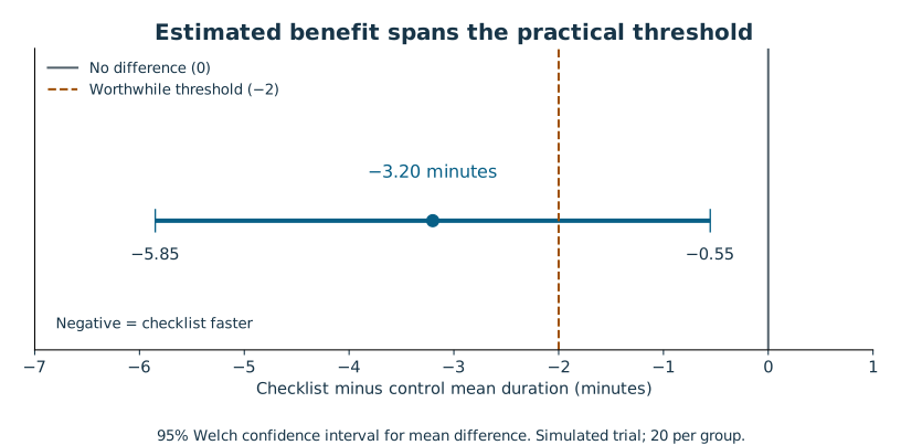
The trial chart shows the mean difference directly. Its interval crosses the hypothetical −2-minute threshold, so a zero-null rejection does not establish that threshold.
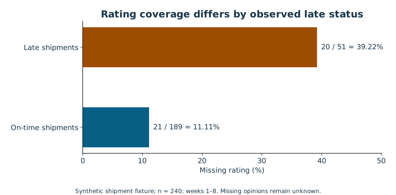
Rating coverage is worse among late shipments in this generated fixture. This does not reveal the unobserved ratings or quantify the exact bias in the all-shipment mean.
Example management brief
Plan a real controlled checklist pilot, and investigate rating-response coverage before using average ratings as a service score. The supplied evidence is a fictional teaching dataset, so it can demonstrate an analysis approach but cannot establish operational effectiveness in a real business.
Across the 240 recorded synthetic shipments in weeks 1–8, 51 were late, or 21.25%. East and West had similar observed late fractions, 25/120 and 26/120 respectively, despite very different average delivery times. East also handled longer routes and a smaller priority-service share. A raw duration ranking therefore does not isolate hub performance. Compare sufficiently overlapping route and service groups and review promise definitions before attributing differences to a hub.
Rating coverage deserves attention: 20 of 51 late shipments lacked ratings, compared with 21 of 189 on-time shipments. The respondent mean of 4.14 therefore describes 199 respondents, with uncertain relevance to all 240 shipments. Investigate response barriers and retain the missingness breakdown alongside any satisfaction headline.
In the separate simulated randomized trial, the checklist mean was 3.20 minutes lower than control. The 95% Welch interval corresponds to a reduction of about 0.55–5.85 minutes. It excludes zero but includes improvements below the hypothetical 2-minute worthwhile threshold. A full rollout is not established as worthwhile, and the fixture measures neither implementation cost nor service-quality trade-offs.
For a real pilot, specify the assignment unit, primary duration outcome, adherence checks, relevant quality guardrails and stopping plan before collecting outcomes. Choose sample size using justified variability and practical-effect assumptions. Review the effect interval against the pre-specified threshold, together with cost and quality evidence. Reconsider the recommendation if the real setting differs materially from the simulated tasks or if quality deteriorates.
Methods and limitations
The optional companion uses exact dependency versions listed in requirements.txt; Python 3.12.14 was tested. Quartiles use NumPy's linear convention and SD uses n−1. The Welch interval and test share the same difference, SE and degrees of freedom. The random generator includes independent normal trial noise with a built-in constant reduction; the observed estimate varies because of assignment/noise. Rounding of CSV durations makes the normal model an excellent teaching approximation rather than literally continuous recorded values.
Shipment summaries are descriptive. They do not receive naive independent-shipment confidence intervals because weekly conditions are shared. Selective missingness is known from the generator but in a real study would require investigation; no exact missing opinions are inferred. A respondent rating mean assumes equal category spacing for that summary and should accompany ordered category counts.
A skeptical reviewer might ask whether a 0.6-minute real reduction would justify adoption. Under the given 2-minute threshold, it would not establish the desired benefit. This is why a zero-null rejection and a worthwhile-intervention decision are not interchangeable. The next study needs relevant outcomes and a design, not simply a larger spreadsheet.