Trace responsibility backward

Outcome: derive every parameter gradient in a scalar network, check it numerically and interpret one update. Prerequisite: Lessons 01–02 and the idea of a slope.

Open the diagram at full size

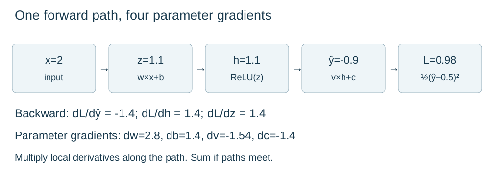
Read the diagram explanation

Forward input 2, preactivation 1.1, ReLU output 1.1, prediction minus 0.9, loss 0.98. Gradient to prediction minus 1.4; parameter gradients: w 2.8, b 1.4, v minus 1.54, c minus 1.4.

A loss says how far a prediction misses its target. It does not directly say which parameter to change. A derivative supplies local information: if one value changes by a small amount while other values stay fixed, how quickly does the loss change? Backpropagation organizes these derivatives through the computation that produced the prediction.

Keep the forward values on the page

Use the same network as Lesson 02: input x = 2, first weight w = 0.5, first bias b = 0.1, output weight v = -1, output bias c = 0.2, and target y = 0.5.

The forward steps are z = w×x + b = 1.1, h = max(0, z) = 1.1, and yhat = v×h + c = -0.9. The loss is L = 0.5×(yhat - y)² = 0.98. Here z is the pre-activation, h the hidden activation, yhat the prediction and L the loss. All four parameters are still at their original values.

We write dL/dw for the derivative of loss with respect to weight w, with the other parameters held fixed. In a multi-parameter setting these are partial derivatives; the collection of them is the gradient. A positive derivative means a sufficiently small increase in that parameter raises this loss locally.

Start at the error and follow each path

The derivative of half-squared error with respect to the prediction is the error itself: dL/dyhat = yhat - y = -1.4. Raising the prediction slightly would lower the loss, which matches the prediction being below the target.

The output is yhat = v×h + c. Increasing v changes the output at rate h = 1.1; increasing c changes it at rate one. The chain rule multiplies the rates along a path:

dL/dv = (dL/dyhat) × h = -1.4 × 1.1 = -1.54
dL/dc = (dL/dyhat) × 1 = -1.4
dL/dh = (dL/dyhat) × v = -1.4 × (-1) = 1.4

At z = 1.1, ReLU is on its positive branch, where changing z changes h at rate one. Therefore dL/dz = 1.4. Finally, the first weighted sum changes at rate x = 2 with respect to w, and at rate one with respect to b:

dL/dw = (dL/dz) × x = 1.4 × 2 = 2.8
dL/db = (dL/dz) × 1 = 1.4

The hidden derivative is positive even though the output derivative is negative. The negative output weight reverses the direction. Memorizing “the error gets sent backward” would miss this multiplication and produce the wrong first-layer update.

Check without trusting the derivation

A central finite difference estimates a derivative by evaluating the loss slightly above and below a parameter value. For weight w, the estimate is [L(w + eps) - L(w - eps)] / (2×eps). eps is a small positive perturbation; all other parameters remain unchanged. We use eps = 0.000001 and double precision to reduce rounding problems.

import math
import torch

values = [0.5, 0.1, -1.0, 0.2]  # w, b, v, c
params = [torch.tensor(t, dtype=torch.float64, requires_grad=True)
          for t in values]
w, b, v, c = params
prediction = v * torch.relu(w * 2.0 + b) + c
loss = 0.5 * (prediction - 0.5) ** 2
loss.backward()

def scalar_loss(p):
    w, b, v, c = p
    prediction = v * max(0.0, w * 2.0 + b) + c
    return 0.5 * (prediction - 0.5) ** 2

eps = 1e-6
expected = [2.8, 1.4, -1.54, -1.4]
for i, (name, parameter) in enumerate(zip(["w", "b", "v", "c"], params)):
    above, below = values.copy(), values.copy()
    above[i] += eps
    below[i] -= eps
    numerical = (scalar_loss(above) - scalar_loss(below)) / (2 * eps)
    automatic = parameter.grad.item()
    assert math.isclose(automatic, expected[i], abs_tol=1e-10)
    assert math.isclose(numerical, automatic, rel_tol=1e-6, abs_tol=1e-8)
    print(name, automatic, numerical)

Autograd records supported tensor operations and uses their derivatives during backward(). It differentiates the computation you wrote, including an incorrectly chosen loss. Numerical agreement is a local implementation check, not proof that the learning problem is well designed.

A perturbation that crosses ReLU's corner at zero can disagree with a single chosen derivative there. Extremely tiny perturbations also invite floating-point cancellation. Our example stays comfortably on the positive branch. Finite differences are useful for tiny checks but would require many forward evaluations for a large parameter set.

One simultaneous update

Plain gradient descent uses new parameter = old parameter - learning_rate×gradient. The learning rate controls the step size. At learning rate 0.1, the four new parameters are w = 0.22, b = -0.04, v = -0.846, and c = 0.34. Every update uses the gradients from the original forward pass; do not recompute only some gradients halfway through.

The new hidden value is max(0, 0.22×2 - 0.04) = 0.4. The new prediction is -0.846×0.4 + 0.34 = 0.0016, giving half-squared loss 0.12420128. Loss decreased on this observation. That alone says nothing about unseen data, and a much larger learning rate could overshoot.

Practice

• 03A · A different target: change only the target to y = -0.5. Derive the original-position loss and all four parameter gradients, then check them with finite differences.
• 03B · A closed gate: set w = -0.5, b = 0.1, keeping x = 2 and the original remaining values. Determine which gradients are zero and explain each zero through its path.
• 03C · Compare step sizes: from the original parameters, calculate one simultaneous update at learning rates 0.01, 0.1 and 1.0. Evaluate each new loss before interpreting which step helped most.

Exit check

Reproduce the four original gradients without code. Then run the numerical check and explain why changing the loss to default MSE doubles those gradients. If signs or factors disagree, identify the first local derivative where your calculation diverges.

Further reading: PyTorch 2.9 Tensor.backward and gradcheck.