Give each training-loop line a job

Outcome: explain and implement a minibatch update, distinguish evaluation mode from disabled gradients, and aggregate loss correctly. Prerequisite: Lessons 01–04.

Open the diagram at full size

Read the diagram explanation

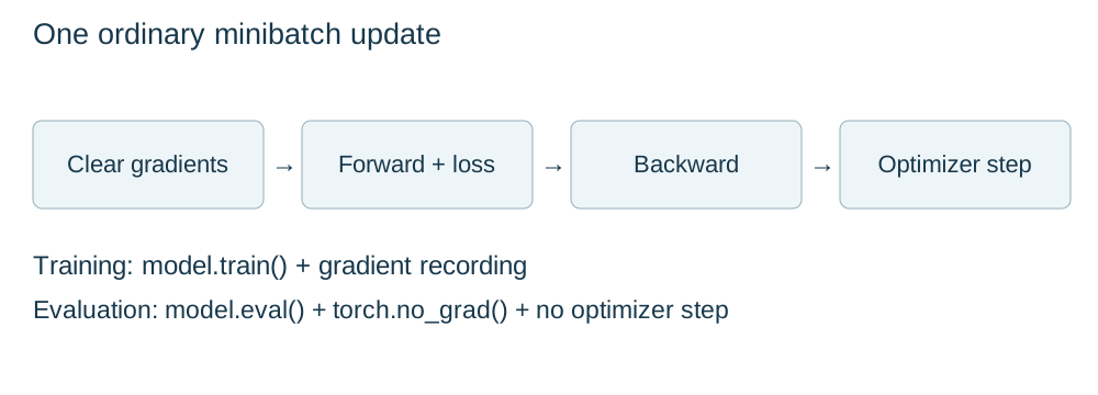
Clear accumulated gradients, compute prediction and loss, backpropagate derivatives, update parameters. Train and evaluation modes are separate from recording gradients.

The training loop repeats the experiment from Lesson 03 on batches. Its brevity can make it tempting to memorize. Instead, follow what changes after each line. Predictions change when parameters change; gradients describe the current computation; and evaluation measures a fixed model without taking an optimization step.

From a gradient to an optimizer

An optimizer receives the parameters it is allowed to update. Plain stochastic gradient descent, or SGD, subtracts the learning rate times each current gradient. “Stochastic” reflects learning from sampled observations or minibatches rather than always using the complete dataset gradient. In our first examples there is no momentum or weight decay, so the update matches the arithmetic already derived.

Create the optimizer once after constructing the model. It must reference the model whose predictions enter the loss. Constructing a second model for the optimizer would leave the first model unchanged. Later optimizers may also retain useful state across steps, making unnecessary reconstruction another source of error.

Read one step in causal order

Start with model.train() to select training behavior. Then optimizer.zero_grad(set_to_none=True) clears gradients left from the previous update. Calculate predictions, calculate the scalar loss, call loss.backward() to obtain gradients, and call optimizer.step() to change parameters.

backward() accumulates into parameter gradients. Without clearing them, a second step can use a mixture of current and stale gradients. Accumulation can be deliberate in more advanced workflows; here it would violate the intended one-batch update. Clearing immediately before each forward pass is an easy convention to audit. Clearing after backward but before the optimizer step discards the gradients the step needs.

The forward pass builds a new computation graph for the current parameters and batch. Do not compute one loss outside the loop and repeatedly call backward on that old computation. Ordinary training does not need retain_graph=True.

A small, complete loop

This miniature linear dataset is an arithmetic diagnostic, separate from the course's held-out sensor experiment. Its four training points follow y = 2×x + 1. There is no claim here about performance on unseen observations.

import torch
from torch import nn
from torch.utils.data import TensorDataset, DataLoader

torch.manual_seed(7)
X = torch.tensor([[-1.0], [0.0], [1.0], [2.0]])
y = 2 * X + 1
loader = DataLoader(TensorDataset(X, y), batch_size=3, shuffle=True,
                    generator=torch.Generator().manual_seed(8))
model = nn.Linear(1, 1)
loss_fn = nn.MSELoss()
optimizer = torch.optim.SGD(model.parameters(), lr=0.05)

for epoch in range(100):
    model.train()
    loss_total, observation_count = 0.0, 0
    for batch_X, batch_y in loader:
        optimizer.zero_grad(set_to_none=True)
        prediction = model(batch_X)
        assert prediction.shape == batch_y.shape
        loss = loss_fn(prediction, batch_y)
        if not torch.isfinite(loss):
            raise RuntimeError("Non-finite training loss")
        loss.backward()
        optimizer.step()
        count = batch_X.shape[0]
        loss_total += loss.item() * count
        observation_count += count
    epoch_training_loss = loss_total / observation_count

model.eval()
with torch.no_grad():
    final_prediction = model(X)
    final_training_mse = loss_fn(final_prediction, y).item()
print("Final training MSE:", final_training_mse)
print("Weight and bias:", model.weight.item(), model.bias.item())

The loop uses default mean MSE with one predicted value per observation. Multiplying each batch mean by its observation count reconstructs its sum of squared errors. Summing those contributions and dividing by the total count gives the correct observed-sample average. If four observations have mean loss one and the final single observation has loss nine, the overall mean is (4×1 + 1×9)/5 = 2.6. Averaging the two batch means would incorrectly give five.

During training, different batches see slightly different parameter values because updates occur between them. The accumulated training loss therefore describes that traversal. Re-evaluating all training observations after the epoch describes the final fixed model, which need not produce the identical number.

Evaluation has two separate switches

model.eval() selects evaluation behavior in layers that distinguish it, including dropout and batch normalization. It does not turn off gradient recording. torch.no_grad() disables gradient recording for operations inside its context, reducing unnecessary tracking during evaluation. It does not select evaluation behavior. Use both when evaluating the course models.

For a network containing only linear layers and ReLU, train/eval mode may not change its predictions. Keeping the distinction explicit prepares you for layers where it matters. Before the next training epoch, call model.train() again. For validation, use the frozen training preprocessing and the validation loader; omit backward and optimizer steps. Test evaluation follows the same computational pattern only after model selection is finished.

Debug the first batch before waiting for epochs

Check prediction shape, target shape, finite values and loss definition first. Inspect a parameter before and after one step to establish that an update occurred. If loss becomes non-finite, investigate inputs, scaling and learning rate before trying a larger network. A simple model should usually be able to fit a tiny, suitable diagnostic dataset, but that test does not measure generalization.

A learning rate that is too large can bounce across useful parameter regions; one that is too small can make progress hard to see. Do not interpret every short-term rise in minibatch loss as failure. Compare epoch-level training and validation behavior while preserving the validation/test roles.

Practice

• 05A · Explain the broken order: consider loss.backward(); optimizer.zero_grad(set_to_none=True); optimizer.step(). Explain what information is discarded and write a correct order for one ordinary update.
• 05B · Weight the final batch: three batches contain four, four and two observations, with mean losses 0.5, 1.0 and 3.0. Compute the full-dataset mean and compare it with the unweighted mean of batch means.
• 05C · Verify a mode distinction: use a Linear(1, 1) model in evaluation mode on an input while gradient recording is enabled. Inspect the output's requires_grad. Repeat inside torch.no_grad() and explain the difference.

Exit check

Run the diagnostic, then explain why a small final training MSE alone is insufficient evidence for deployment. On a fresh single batch, show that gradients exist after backward and at least one parameter changes after the optimizer step.

Further reading: PyTorch 2.9 SGD, zero_grad, module modes, and no_grad.