A tiny convolutional network you can account for

Flattening an image makes it usable by an ordinary linear layer, but it discards explicit neighborhood structure. Pixel 17 and pixel 18 may be adjacent; pixel 17 and pixel 49 may not be. A convolutional layer applies a small learned pattern detector repeatedly across local neighborhoods. Reusing the same weights across positions is the key structural assumption. A horizontal edge should be recognizable in more than one part of an image.

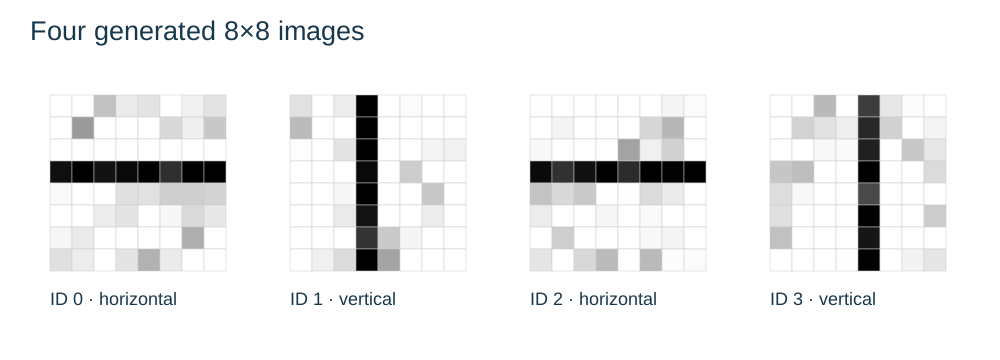
We use 8-by-8 grayscale images generated entirely in the course. Each image contains a noisy horizontal or vertical bright bar. Class 0 is horizontal; class 1 is vertical. Positions vary, noise is independent and pixel values are clipped to known bounds 0–1. This dataset is intentionally small enough to inspect, generate and train on CPU. It does not stand in for medical images, handwriting or real camera scenes.

Open the diagram at full size

Read the diagram explanation

First four fixture images alternate horizontal and vertical noisy bars. Darker display pixels indicate larger numerical intensity; labels describe orientation.

Compute one local response

Consider the 3-by-3 image patch with rows [0,0,0], [1,1,1], [0,0,0]. A horizontal-line kernel with the same three rows produces response 3: multiply corresponding entries and add them. A vertical-line kernel with rows [0,1,0], [0,1,0], [0,1,0] produces response 1 on that patch. A bias, if present, is added after the sum. The numbers illustrate a possible detector; actual training learns its own weights and need not reproduce these exact kernels.

PyTorch calls the layer Conv2d, though its numeric operation is cross-correlation: it does not flip the kernel as a strict mathematical convolution definition would. This distinction matters when checking arithmetic by hand, but the learned-weight idea is the same.

A channel is one feature plane. Grayscale input has one channel. Four learned kernels produce four output channels, each potentially responsive to a different pattern. More channels are not more training examples. The batch axis still counts examples.

Account for every dimension

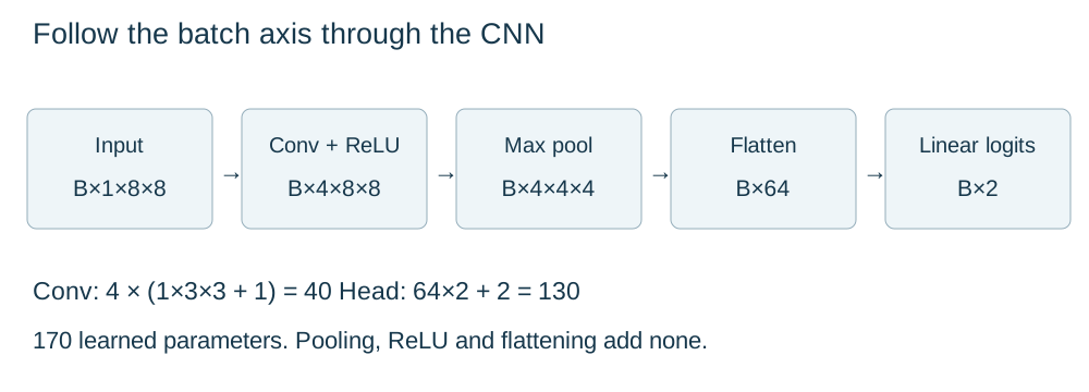
The model uses Conv2d(1,4,kernel_size=3,padding=1), ReLU, MaxPool2d(2), flattening and a linear head. For batch size 5:

• Input: [5,1,8,8]
• Convolution: [5,4,8,8]
• ReLU: [5,4,8,8]
• Two-by-two max pooling with stride 2: [5,4,4,4]
• Flatten from dimension 1: [5,64]
• Linear layer to two class logits: [5,2]

With dilation 1, output width is floor((input_width + 2*padding - kernel_width)/stride) + 1. Here it is (8+2-3)/1+1 = 8. Without padding, it would be 6. Max pooling keeps the greatest value in each non-overlapping two-by-two neighborhood. That reduces resolution; it can preserve a strong local response while losing its exact position. Pooling does not guarantee invariance to every shift, and boundaries still matter.

Open the diagram at full size

Read the diagram explanation

Input shape batch by 1 by 8 by 8; convolution has 4 channels; pooling gives 4 by 4; flatten gives 64; linear head gives two logits. Forty convolution and 130 linear parameters.

Count parameters rather than guessing from layer count. Each convolutional output channel has 1*3*3 = 9 weights and one bias. Four channels give 40 parameters. The linear head has 64*2 = 128 weights and two biases, giving 130. Total: 170. ReLU, max pooling and flattening have no learned parameters. python -m examples.04_cnn_shapes checks both dimensions and count.

Train with the same experimental discipline

The targets are integer class indices, so the head returns raw logits and the loss is CrossEntropyLoss. Do not add a final softmax before that loss. Softmax is useful when presenting relative class probabilities after training. Argmax of logits already gives the same most-probable class without an extra softmax calculation.

Run python -m dlcourse.run --task bars. The declared candidates are a flattened linear classifier and the tiny CNN. Each uses only training rows for updates, validation loss selects its checkpoint, and the winning candidate is selected before the test calculation. The flattened baseline matters: if a simple model works as well, a CNN may not be necessary for this task. More complicated architecture is not an automatic achievement.

Inspect false positives and false negatives on validation. Ask whether errors depend on bar position or noise, and whether a proposed augmentation preserves labels. Horizontal or vertical translation can preserve orientation. A 90-degree rotation swaps horizontal and vertical, so retaining the old label would corrupt this particular task. Augmentation is a statement about the meaning of the target, not a universal checklist.

Exercises

• 9A · Local detector. Compute the horizontal and vertical kernel responses on a vertical center-column patch. Assume zero bias.
• 9B · Shape change. Remove convolution padding but keep the rest of the architecture. Find the new feature shape after pooling and the required input dimension of the final linear layer.
• 9C · Label-preserving transforms. Classify horizontal flip, 90-degree rotation and mild added sensor noise as safe, label-changing or assumption-dependent for this dataset. Explain each decision.

Exit check: derive the 170-parameter count without running code, and state why success on these generated bars does not validate real-world computer vision.