Ask what extra flexibility actually buys

Outcome: compare a linear baseline with a small nonlinear model using a fixed evaluation plan, and explain the geometry of a ring classifier. Prerequisite: Lessons 01–05 and baseline evaluation from Applied Machine Learning.

Open the diagram at full size

Read the diagram explanation

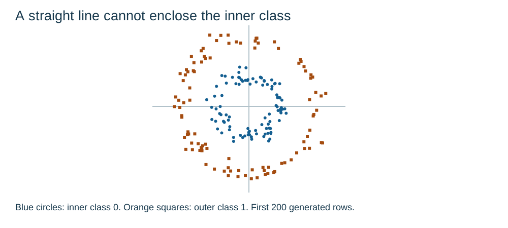
Scatter of the first 200 generated points. Inner class shown as blue circles, outer class orange squares. Both axes arbitrary feature units; horizontal and vertical scales are equal.

A deeper model is useful only when its additional flexibility addresses a relevant limitation and survives evaluation. Begin with a model simple enough to understand. It establishes a reference score and exposes data or training problems that additional layers could hide. This lesson joins two small questions: predicting a continuous sensor response and classifying concentric rings.

First establish the regression baseline

The sensor fixture relates two measured inputs to a continuous response, with a squared effect of the first input and independent noise. Fit an intercept-only reference using the training-target mean, then fit a linear regression model using Linear(2, 1) and MSELoss. Both use the same fixed split IDs. Standardize both features using training statistics; keep the target in its original units so the error remains interpretable.

The constant reference asks how much improvement comes from using the input at all. The linear model asks how much a straight trend captures. Calculate validation MSE for selection and, when reporting results, also consider mean absolute error, the average absolute prediction error. MSE squares target units; mean absolute error retains the target's units. Neither describes the cause of the relationship.

To see a linear limitation without training anything, take hypothetical inputs [-1, 0, 1] and targets [1, 0, 1]. A constant prediction of 2/3 gives squared errors 1/9, 4/9 and 1/9; mean error is 2/9. Symmetry makes the best least-squares line horizontal here. Increasing training time cannot make that line bend downward in the middle.

These three points are an arithmetic illustration, not a claimed score on the sensor fixture. On actual validation observations, inspect residuals as well as an average. Residual means observed target minus prediction. A curved residual pattern provides a specific reason to consider a nonlinear candidate. A larger model's lower training error alone does not.

Hidden units make several local rules possible

A multilayer perceptron, abbreviated MLP, combines affine layers with nonlinear activations. With one hidden layer, each hidden unit receives a weighted sum of the input and applies ReLU. The final layer combines the resulting activations.

For one input, ReLU creates a change of slope where its weighted input crosses zero. Several hidden units can place changes at different positions, approximating a curve over the observed range. In two dimensions, these become changes across regions. Extrapolation still needs separate justification.

import torch
from torch import nn

linear_regressor = nn.Linear(2, 1)
linear_classifier = nn.Linear(2, 1)
ring_classifier = nn.Sequential(
    nn.Linear(2, 16), nn.ReLU(),
    nn.Linear(16, 16), nn.ReLU(), nn.Linear(16, 1),
)

assert linear_regressor(torch.zeros(4, 2)).shape == (4, 1)
assert linear_classifier(torch.zeros(4, 2)).shape == (4, 1)
assert ring_classifier(torch.zeros(4, 2)).shape == (4, 1)
assert sum(p.numel() for p in ring_classifier.parameters()) == 337

Sequential passes each layer's output into the next. This course comparison uses two hidden layers: 48 parameters in the first layer, 272 in the second and 17 in the output, totaling 337. The linear classifier has three. The regression MLP uses the same dimensions but a different loss. Extra parameters create flexibility and additional estimation demands.

Why rings are a useful challenge

Each ring observation has two coordinate features. One class lies near an inner circle and the other near an outer circle, with independently generated variation. A one-logit linear classifier predicts from a×x1 + b×x2 + c. Here x1 and x2 are the two coordinates, a and b are their weights, and c is a bias.

At the default probability threshold 0.5, a zero logit marks the boundary. The equation a×x1 + b×x2 + c = 0 describes a straight line when the feature weights are not both zero. A straight line cannot surround the inner ring while excluding the outer ring everywhere. Training longer cannot remove that representational limitation.

ReLU hidden units combine several regions, allowing a small MLP to approximate an enclosing boundary. Train it with BCEWithLogitsLoss using floating-point binary labels shaped (B, 1). For a default label prediction, compare its logit with zero; apply sigmoid only when you need a displayed probability. Keep any threshold choice part of validation-based selection, not test-based adjustment.

Compare procedures, not lucky runs

Keep split IDs, preprocessing rules, metric definitions and the candidate budget fixed. Record the model, initialization seed, learning rate, batch size and stopping rule. Use validation results to choose between candidates and restore the selected parameter state before the final test. If early stopping is used, the final training epoch may not contain the selected model.

The supplied comparison selects by validation loss. Also compare accuracy with a majority-class reference chosen from training labels. Inspect a confusion matrix: true/predicted class counts can expose neglect of one class. These synthetic results do not certify real-world performance.

Use a small, declared candidate set. Repeated validation selection can overfit the development evidence. Test once after fixing the procedure and report the result without silently replacing inconvenient outcomes.

Practice

• 06A · Count a smaller candidate: count the parameters in Linear(2, 1) and in a 2–16–1 MLP with ReLU. Compare the latter with the displayed 2–16–16–1 model. Explain which additional capability depends on ReLU.
• 06B · Explain the boundary: sketch ideal circles of radii one and two. Draw a straight decision boundary, identify where it must fail, and describe why a collection of piecewise-linear regions could help.
• 06C · Make a selection plan: specify a comparison of the linear and MLP ring classifiers, including fixed data, training-only preprocessing, one primary validation metric, a stopping rule and the point at which the test set may be evaluated. Do not invent performance numbers.

Exit check

Explain a plausible observation that would justify trying the MLP and one that would make you investigate the pipeline first. For each candidate, state its exact output/loss contract and identify the evidence needed before claiming an improvement.

Further reading: PyTorch 2.9 Sequential and Linear; scikit-learn's common evaluation pitfalls.