Describe a typical value and what it hides

A manager has time to hear one number. Which one should you choose? That depends on the decision. If you need total labor minutes for six jobs, the mean connects directly to the total. If you want to describe an ordinary job when a few jobs take much longer, the median may give a more useful sense of the center. Neither number replaces the distribution.

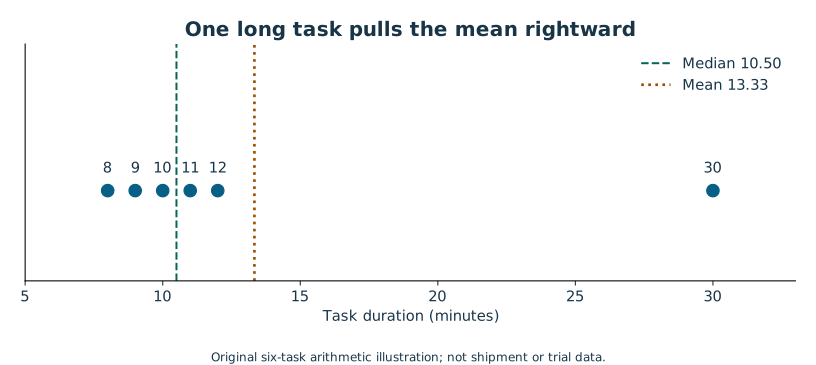
Consider six fictional task durations in minutes: 8, 9, 10, 11, 12 and 30. We use this deliberately small list so you can check every calculation without writing code. It is a separate arithmetic example, not a subset of the shipment file.

Two honest centers, two different questions

Add the durations: 8 + 9 + 10 + 11 + 12 + 30 = 80. Divide by six to obtain a mean of 13.333… minutes. If all six jobs had taken that long, their total would still be 80 minutes. The mean is a balance point for the total, so the 30-minute job pulls it upward.

For the median, sort the observations first. There are six values, so the middle lies between the third and fourth: (10 + 11) / 2 = 10.5 minutes. The median describes a middle position, not a share of the total. Five of these six jobs are shorter than the mean, which is possible because the mean is not defined as the halfway-ranked value.

If the longest job changes from 30 to 60, the mean rises to 18.333… minutes while the median remains 10.5. That does not prove the median is always “better.” A planner paying for all the minutes needs to account for the long job. A user asking about a typical wait should also hear about the tail. A useful sentence is “The median was 10.5 minutes; the mean was 13.3 because one of six jobs took 30 minutes.”

Spread makes the center useful

The range is 30 − 8 = 22 minutes. It shows the endpoints but ignores the other four values. The interquartile range, or IQR, focuses on the middle of the ranked data. We use NumPy's linear interpolation convention throughout, because software packages can disagree on quartiles for small samples.

For six sorted values, the zero-based position of the 25th percentile is (6 − 1) × 0.25 = 1.25. Position 1 is 9 and position 2 is 10. Move one quarter of the way from 9 to 10: Q1 is 9.25. The 75th-percentile position is 3.75, between 11 and 12, giving Q3 = 11.75. The IQR is 11.75 − 9.25 = 2.5 minutes. A different documented convention can give a different correct answer; silently mixing conventions cannot.

Standard deviation uses all the values. First find how far each observation is from the mean. Square those deviations so positives and negatives do not cancel. Their sum here is 343.333… squared minutes. For the sample variance, divide by n − 1 = 5, obtaining 68.666… squared minutes. Take the square root to return to minutes: the sample standard deviation is 8.287 minutes. You do not need to memorize the squared deviations; understand that far-away points receive substantial weight.

We use the sample standard deviation, denoted s, in the inferential examples because the observed sample is being used to estimate a process's variation. Dividing by n instead describes the variance of those particular listed values as a complete finite population. State which convention you used. Standard deviation describes variation among individual observations. It is not the uncertainty of the sample mean; that distinction arrives in Lesson 6.

Open the diagram at full size

Read the diagram explanation

Values 8, 9, 10, 11, 12, 30 minutes. Median 10.5, mean 13.333. The longest value pulls the mean above the median.

An outlier flag is a question

A common boxplot fence puts a flag above Q3 + 1.5 × IQR. Here the upper fence is 11.75 + 3.75 = 15.5 minutes. The 30-minute job is flagged. The rule does not establish that it is a mistake, a statistically impossible event, or a record you are allowed to delete.

Ask what happened. Perhaps a timestamp was entered incorrectly. Perhaps the job was genuinely difficult. If an independently verified correction exists, record the correction and its provenance. If the value is plausible and unverified, retain it in the primary result. You can report a sensitivity comparison with and without it, clearly labelled, to show how much it influences the conclusion. Removing it would reduce this example's mean to 10 minutes. Reporting only that smaller number would misrepresent the original six jobs.

A long right tail means some large values stretch the distribution. It is not a diagnosis. Mixed task types can create that tail, and a logarithmic scale or a more robust summary may help exploration. Neither transformation nor trimming should be chosen after seeing which version makes a preferred story look strongest.

Apply the reasoning to the shipment file

For actual delivery time, report the count, mean, median, sample SD, IQR and range together during exploration. Do not call a delivery “bad” solely because it is far from the average: distance and promise matter. For ratings, report the ordered category counts and missing count before choosing a mean. These summaries let another person see what a single headline number conceals.

Attempt Practice 2A–2C. Explain why deleting the 30-minute value is a substantive decision, and why an average rating of 4 does not imply most people selected 4.

Further reading: NIST on location, NIST on spread, NumPy's quantile methods, and NIST on investigating outliers.