
Statistics · Module 5
Reason about probability without losing the denominator
Probability gives us a language for uncertainty. Probabilities range from 0 to 1. In our finite counting examples, 0 means no favorable cases and 1 means all cases are favorable. Continuous models need more care: an exact value can have probability zero without being impossible. Between the endpoints, the value describes how much chance the model assigns to an event. An observed proportion is a count divided by a count. It can inform a probability model, but it is not a guarantee about the next case.
In the supplied shipment file, 51 of 240 shipments are late. The observed fraction is 51/240 = 0.2125, or 21.25%. If you selected one of these 240 rows uniformly at random, the probability it is a late row would be exactly 21.25%. If you asked whether tomorrow's first real delivery would be late, this fictional file would provide no real-world evidence. Even in a genuine operation, that prediction would require assumptions about how tomorrow resembles the recorded period.
Complement and conditional probability
If late and on-time are exhaustive categories with no unknown status, the on-time probability is 1 minus the late probability. In a separate model with late probability 0.20, the on-time probability is 0.80. If unknown statuses exist, “not known to be late” is not the same as “known to be on time.” Define the categories before subtracting.
Conditional probability means restricting attention to a condition. Suppose a tiny invented table has 100 deliveries: 20 priority, of which 4 are late, and 80 standard, of which 24 are late. The late rate among priority deliveries is 4/20 = 20%. The priority share among late deliveries is 4/28 ≈ 14.29%. Both are valid, but the denominators answer different questions. Read “among” as an instruction to define the denominator.
The joint probability of being both priority and late in this table is 4/100 = 4%. It also equals the priority share, 20/100, multiplied by the late fraction within priority, 4/20. The middle count cancels: (20/100) × (4/20) = 4/100. This multiplication uses a conditional probability, so it does not assume independence.
Independence is a claim, not a default
Two events are independent when learning that one occurred does not change the probability of the other under the model. Only then can you multiply their separate probabilities directly. If two independent shipments each have a 0.20 chance of being late, the chance both are late is 0.20 × 0.20 = 0.04. The chance at least one is late is easier through the complement: 1 − 0.80 × 0.80 = 0.36.
Shared road closures or weather could make real shipment outcomes dependent. The independence calculation would then be inappropriate. Our observational fixture includes shared weekly conditions, so the two-shipment calculation is explicitly a separate toy model. Never carry an assumption from an easy example into a new dataset without checking the design.
A base-rate example you can count
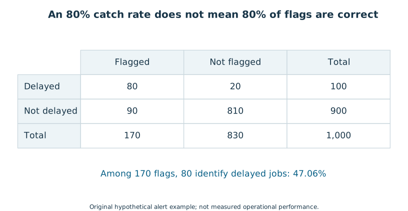
Imagine a fictional alert system evaluated on 1,000 jobs. Exactly 100 are truly delayed. It flags 80 of those 100, and it also flags 90 of the 900 jobs that are not delayed. The system catches 80% of delayed jobs, but a flagged job is not delayed with 80% probability.
| Actual state | Flagged | Not flagged | Total |
|---|---|---|---|
| Delayed | 80 | 20 | 100 |
| Not delayed | 90 | 810 | 900 |
| Total | 170 | 830 | 1,000 |
Among all 170 flags, only 80 represent delayed jobs: 80/170 ≈ 47.06%. The many non-delayed jobs create 90 false alarms even though only 10% of that group is flagged. The underlying prevalence, 100/1,000, is called a base rate. Ignoring it can turn a technically correct performance statement into an incorrect operational expectation.
Read the diagram explanation
Hypothetical 1,000 jobs: 100 delayed, 900 not. Flags identify 80 delayed and 90 not delayed. 80 of 170 flagged jobs are delayed, or 47.06%.
A manager deciding whether to investigate each flag needs the expected workload and false-alarm burden, not just the catch rate. If investigation costs 2 minutes per flag, these 170 flags require 340 minutes in this example. That is arithmetic under an explicitly supplied cost assumption, not a cost estimate for the shipment operation.
From individual outcomes to distributions
A binary late outcome has two possible values, 0 and 1. A count of late outcomes across independent trials with the same late probability follows a binomial model. Actual delivery minutes vary on a numerical scale and usually require a different model. Not every measurement is bell-shaped, and the fact that software offers a normal distribution is not evidence that your data follows it.
You now have enough probability vocabulary for sampling uncertainty: an event, a probability under a model, a condition, independence and a distribution of possible outcomes. Attempt Practice 5A–5C. The most important habit is to write the denominator in words before calculating a percentage.
Further reading: NIST's binomial model. The alert example is an original, fully specified counting exercise.
Read the separate answers and explanations
Reading progress
12 lessons remain open to guests. Marking a lesson read records reading only; it does not award assessment credit or a certificate.
Device reading marks require browser storage. Reading is always available.
Sign in or create an account to save separate account progress. Your current page is kept.
Your earlier place on this device suggests these lessons. No new lesson is marked read.